


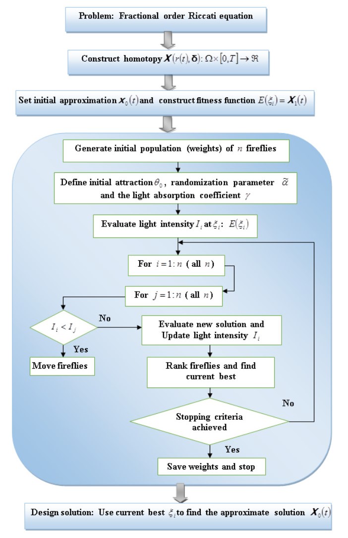
Figure 1.
Generic flow diagram of the expedite homotopy perturbation method.
Citation: Nora Aïssiouene, Marie-Odile Bristeau, Edwige Godlewski, Jacques Sainte-Marie. A combined finite volume - finite element scheme for a dispersive shallow water system[J]. Networks and Heterogeneous Media, 2016, 11(1): 1-27. doi: 10.3934/nhm.2016.11.1
| [1] | Manal Alqhtani, Khaled M. Saad, Rasool Shah, Thongchai Botmart, Waleed M. Hamanah . Evaluation of fractional-order equal width equations with the exponential-decay kernel. AIMS Mathematics, 2022, 7(9): 17236-17251. doi: 10.3934/math.2022949 |
| [2] | Rasool Shah, Abd-Allah Hyder, Naveed Iqbal, Thongchai Botmart . Fractional view evaluation system of Schrödinger-KdV equation by a comparative analysis. AIMS Mathematics, 2022, 7(11): 19846-19864. doi: 10.3934/math.20221087 |
| [3] | Azzh Saad Alshehry, Naila Amir, Naveed Iqbal, Rasool Shah, Kamsing Nonlaopon . On the solution of nonlinear fractional-order shock wave equation via analytical method. AIMS Mathematics, 2022, 7(10): 19325-19343. doi: 10.3934/math.20221061 |
| [4] | Naveed Iqbal, Muhammad Tajammal Chughtai, Nehad Ali Shah . Numerical simulation of fractional-order two-dimensional Helmholtz equations. AIMS Mathematics, 2023, 8(6): 13205-13218. doi: 10.3934/math.2023667 |
| [5] | Samia Bushnaq, Sajjad Ali, Kamal Shah, Muhammad Arif . Approximate solutions to nonlinear fractional order partial differential equations arising in ion-acoustic waves. AIMS Mathematics, 2019, 4(3): 721-739. doi: 10.3934/math.2019.3.721 |
| [6] | Yousef Jawarneh, Humaira Yasmin, M. Mossa Al-Sawalha, Rasool Shah, Asfandyar Khan . Fractional comparative analysis of Camassa-Holm and Degasperis-Procesi equations. AIMS Mathematics, 2023, 8(11): 25845-25862. doi: 10.3934/math.20231318 |
| [7] | Manoj Singh, Ahmed Hussein, Msmali, Mohammad Tamsir, Abdullah Ali H. Ahmadini . An analytical approach of multi-dimensional Navier-Stokes equation in the framework of natural transform. AIMS Mathematics, 2024, 9(4): 8776-8802. doi: 10.3934/math.2024426 |
| [8] | Sumbal Ahsan, Rashid Nawaz, Muhammad Akbar, Saleem Abdullah, Kottakkaran Sooppy Nisar, Velusamy Vijayakumar . Numerical solution of system of fuzzy fractional order Volterra integro-differential equation using optimal homotopy asymptotic method. AIMS Mathematics, 2022, 7(7): 13169-13191. doi: 10.3934/math.2022726 |
| [9] | M. M. Khader, A. M. Shloof, Halema Ali Hamead . Numerical investigation based on the Chebyshev-HPM for Riccati/Logistic differential equations. AIMS Mathematics, 2025, 10(4): 7906-7919. doi: 10.3934/math.2025363 |
| [10] | Muath Awadalla, Abdul Hamid Ganie, Dowlath Fathima, Adnan Khan, Jihan Alahmadi . A mathematical fractional model of waves on Shallow water surfaces: The Korteweg-de Vries equation. AIMS Mathematics, 2024, 9(5): 10561-10579. doi: 10.3934/math.2024516 |
In the past few years, fractal calculus and fractional calculus has been one of the most rapidly growing areas of mathematical analysis, which are used to model various problems of real life. Fractal calculus is considered as a fruitful field of research in science and technology and is extensively used to elucidate the phenomena of hierarchical or porous media [1]. Owing to the simplicity and effectiveness of fractal derivative it has defined an alternative approach of fractional derivatives, to explain some of the most fundamental theories with considerable ease and elegance [2,3]. The fractional derivative and fractional integral operators are the valuable tools which are used in the modeling of various physical phenomena of science and engineering. Anomalous dynamics of numerous complex nonlinear systems are elegantly modeled by the assistance of fractional differential equations, which are acknowledged as the generalization of the classical differential equations of integer order [4,5,6].
The fractional order Ricatti equation (RE) accommodates an extremely significant class of nonlinear differential equations which includes: The nth order linear homogenous ODE, one-dimensional Schrödinger equation, wave solution of nonlinear partial differential equation (PDE), etc [7]. These REs has substantial importance in classical, as well as, modern science and engineering problems because of their multifarious applications in various fields. For instance, optimal control, variational calculus, random processes, quantum mechanics, thermodynamics, robust stabilization, stochastic realization theory and diffusion problems [8,9,10,11].
The mathematical formulation for the nonlinear Ricatti differential equations with the fractional derivative defined in the Caputo sense is read as,
| CDα0x(t)=p(t)x2(t)+q(t)x(t)+r(t),0⩽t⩽T | (1) |
with the initial condition defined as,
| x(t0)=η, | (2) |
where, α is the order of equation, α>0 and α∈ℜ, with T,t0,η∈ℜ; p(t),q(t),r(t) are the real continuous functions and x(t)is the solution of the equation. The behavior of the aforementioned Eq. (1) depends on the parameter α, which can be varied to analyze the dynamical behavior of these equations. In order to study the nonlinear Eq. (1) various analytical and numerical techniques developed in the past were applied by many researchers and scientists to compute the solutions of these equations among which some of them are cited here: The homotopy perturbation method (HPM) [12], the fractional-order Legendre operational matrix method [13], the iterative reproducing kernel Hilbert space method [14], the optimal homotopy asymptotic method [15], the modified Laplace Adomian decomposition method [16], the B-spline operational method [17] and the Haar wavelet collocation method [18]. The HPM introduced by He has been successfully used to solve numerous linear and nonlinear problems of real life. Since, its development it has been modified by He and many other scientists to solve various ordinary and partial differential equations of integer and non-integer order [19,20,21].
The demand of global optimization technique is increasing day by day, which are utilized in the assessment of numerous nonlinear and multimodal problems of real life. The deterministic algorithm and the stochastic algorithm are the two types of optimization algorithm that are found in the literature [22,23]. The deterministic algorithm are often gradient-based whereas, the stochastic algorithm are further subcategorized as heuristic or metaheuristic algorithm. In recent trends, the popularity and demand of the nature inspired algorithms have increased extensively. Nature inspired metaheuristic algorithms which efficiently deals with the nonlinear optimization problems includes the genetic algorithm (GA) [24], simulated annealing (SA) algorithm [25], differential evolution (DE) algorithm [26], the ant colony optimization (ACO) algorithm [27], particle swarm optimization (PSO) algorithms [28], the shark smell algorithm [29] and the most powerful and demanding firefly (FA) algorithm [30,31,32].
The FA which mimics the flashing pattern and behavior of the fireflies was first developed by Yang in 2008 and since then it has been modified by various scientist and researcher to solve different types of challenging optimization problems. Some of the flashing characteristic of these unisex fireflies are idealized to develop the FA. The three idealized rule used by the firefly algorithm are as follows:
● A firefly is attracted to the other fireflies regardless of their gender.
● Attractiveness of fireflies is directly proportional to their brightness. The attractiveness and brightness of fireflies both increases as the distance between them deceases.
● Brightness of a firefly is determined by the objective function.
The literature of this modern, self-adaptive, highly efficient and truly intelligent algorithm has expanded dramatically [30,31,32,33,34].
The fundamental aim of this paper is to provide a numerical technique for the assessment of nonlinear fractional differential model defined as (1) and (2). The concept of classical homotopy perturbation method is merged with the modern metaheuristic optimization technique for the development of an expedite homptopy perturbation method (EHPM). The developed method-EHPM transforms the fractional model into a system of algebraic equations leading to a fitness function determined by a particular fragment of the weighted series solution, which are trained by the using the powerful and reliable optimization technique-FA. The optimal values achieved by the FA are utilized to attain the accurate, convergent and reliable solutions. Comparative study is conducted by the comparing the EHPM computed results with the available exact solution and the solutions obtained by the modified homotopy perturbation (MHPM) [35], the residual power series method (RPSM) [36] and the Adam bashforth method (ABMA) [37]. Furthermore, the accuracy and competency of the EHPM is also ratified by computing results by the proposed design methodology in combination with accelerated particle swarm optimization (APSO), i.e., the fitness function determined by EHPM is optimized by using APSO. Various error measures are also carried out to validate the correctness and accuracy of the suggested scheme.
Some basic definitions of the fractional calculus which are going to be utilized in the further discussion are stated below:
Definition 2.1. Let f(x) be a differential function with β∈(0,1],then the Caputo order fractional derivative CDβ0f(x), is defined as [36],
| CDβ0f(x)={1Γ(1−β)x∫0(x−ϖ)−βf′(ϖ)dϖ,0<β<1,df(x)dx,β=1, | (3) |
with CDβ0ω=0, for some constant ω∈R.
Definition 2.2. For any function f(x) with x:[0,∞)→ℜ, the Riemann fractional integral of order β is given as [35],
| RIβ0f(x)=1Γ(β)x∫0(x−ϖ)β−1f(ϖ)dϖ, | (4) |
where β>0 and β∈ℜ.
This section comprehensively describes the procedure to determine the approximate solutions of the nonlinear fractional differential equations using the classical idea of HPM with the modern optimizing tool. A brief review of the learning solver FA, which is utilized for the development of the presented scheme (EHPM) is also demonstrated here.
To exemplify the basic ideas of the proposed scheme consider the nonlinear FDE of the form,
| ψ|(x,t,g)=0,Ω=[0,T]∈ℜ | (5) |
with the initial condition defined as
| x(t0)=η,η,t0∈ℜ, | (6) |
where g and xare function of t and Ω is the boundary of the domain. Then \rm{ \mathit{ ψ}} can be expressed as
| {\bf{L}}\left( {x,t} \right) + {\bf{N}}\left( {x,t} \right) + {\bf{A}}\left( {g\left( t \right)} \right) = 0, | (7) |
Where L is the linear operator, N is the nonlinear operator and A is the known analytical function. By the homotopy procedure we rewrite Eq. (7) as
| \mathit{\boldsymbol{H}}\left( {\mathit{\boldsymbol{X}}\left( t \right)\mathit{\boldsymbol{, }}{\bf{ {{ δ}} }}} \right) \equiv {\bf{L}}\left( {\mathit{\boldsymbol{X}}\left( t \right), t} \right) - {\bf{L}}\left( {{\mathit{\boldsymbol{x}}_\mathit{\boldsymbol{0}}}\left( t \right), t} \right) + {\bf{ {{ δ}} }}{\bf{L}}\left( {{\mathit{\boldsymbol{x}}_0}\left( t \right), t} \right) + {\bf{ {{ δ}} }}\left( {{\bf{N}}\left( {\mathit{\boldsymbol{X}}\left( t \right), t} \right) + {\bf{A}}\left( {g\left( t \right)} \right)} \right) = 0 | (8) |
where {{\mathit{\boldsymbol{x}}_0}\left(t \right)} is an initial approximation, and {\bf{ {{ δ}} }} is an embedding parameter defined in some closed interval \left[{0, 1} \right]. Let the homotopy solution of equation Eq. (8) can be written as
| \mathit{\boldsymbol{X}}\left( t \right) = \sum\limits_{k = 0}^\infty {{{\bf{ {{ δ}} }}^k}{\mathit{\boldsymbol{X}}_k}\left( t \right)} | (9) |
where {{\mathit{\boldsymbol{X}}_k}\left(t \right)} are attained by the kth-order homotopy derivative defined as
| {\mathit{\boldsymbol{X}}_k}\left( t \right) = \frac{1}{{k!}}{\left. {\frac{{{\partial ^k}\mathit{\boldsymbol{H}}}}{{\partial {{\bf{ {{ δ}} }}^k}}}} \right|_{{\bf{ {{ δ}} }} = 0}} | (10) |
Now, we let the initial approximation of Eq. (8) of the form
| {\mathit{\boldsymbol{x}}_0}\left( t \right) = \sum\limits_{i = 0}^n {\frac{{{t^{i\alpha }}{\xi _i}}}{{\Gamma \left( {i\alpha + 1} \right)}}} | (11) |
where {\xi _0}, {\xi _1}, {\xi _2}, \ldots, {\xi _n} are the unknown weights to be determined. By utilizing the Eq. (11), Eq. (9) and the basic ideas of MHPM [35] with {\mathit{\boldsymbol{X}}_1}\left(t \right) = 0 and {\mathit{\boldsymbol{L}}^{\mathit{\boldsymbol{ - 1}}}} as the inverse operator of L we obtain an algebraic system expressed as
| {\mathit{\boldsymbol{X}}_0} = {\mathit{\boldsymbol{L}}^{ - 1}}\left( {\sum\limits_{i = 0}^n {\frac{{{t^{i\alpha }}{\xi _i}}}{{\Gamma \left( {i\alpha + 1} \right)}}} } \right) | (12) |
| {\mathit{\boldsymbol{X}}_1}\left( t \right) = {\mathit{\boldsymbol{L}}^{\mathit{\boldsymbol{ - 1}}}}\left( {{\bf{L}}\left( {{\mathit{\boldsymbol{x}}_0}\left( t \right), t} \right) + {\bf{N}}\left( {\mathit{\boldsymbol{X}}\left( t \right), t} \right) + {\bf{A}}\left( {g\left( t \right)} \right)} \right) | (13) |
and {\mathit{\boldsymbol{X}}_2}\left(t \right) = {\mathit{\boldsymbol{X}}_3}\left(t \right) = \ldots = 0. Setting {\mathit{\boldsymbol{X}}_1}\left(t \right) = 0 by MHPM, automatically leads the solution of Eq. (8) written as:
| x\left( t \right) = X\left( t \right) = {\mathit{\boldsymbol{X}}_0} = {\mathit{\boldsymbol{L}}^{ - 1}}\left( {\sum\limits_{i = 0}^n {\frac{{{t^{i\alpha }}{\xi _i}}}{{\Gamma \left( {i\alpha + 1} \right)}}} } \right) | (14) |
The aforementioned approximate solution (14) comprises of the unknown weights {\xi _0}, {\xi _1}, {\xi _2}, \ldots, {\xi _n} which are determined by constructing a fitness function given as
| E\left( {{\xi _i}} \right) = \min \sum\limits_{j = 1}^m {\left| {{\mathit{\boldsymbol{X}}_1}\left( {{t_j}} \right)} \right|} | (15) |
The weights in Eq. (15) are learned by using a modern and powerful optimization technique FA. The graphical abstract of the above presented scheme EHPM is portrayed in Figure 1.
Lemma 3.1. In problem (5) if x\left(t \right) = {\mathit{\boldsymbol{X}}_\mathit{\boldsymbol{0}}} is the solutions of Eq. (9), which comprises of the unknown weights {\xi _i}\begin{array}{*{20}{c}}; \end{array}i = 0, 1, 2, ..., n, then the minimization problem will be simplified as:
| E\left( {{\xi _i}} \right) = \min \sum\limits_{j = 1}^m {\left| {\left( {{t_j}, {\mathit{\boldsymbol{X}}_\mathit{\boldsymbol{0}}}\left( {{t_j}, {\xi _i}} \right), D_t^\alpha {\mathit{\boldsymbol{X}}_\mathit{\boldsymbol{0}}}\left( {{t_j}, {\xi _i}} \right)} \right)} \right|} | (16) |
Theorem 3.2. If the solution of Eq. (8) satisfies {\mathit{\boldsymbol{X}}_1}\left(t \right) = 0, then Eq. (10) results {\mathit{\boldsymbol{X}}_2}\left(t \right) = {\mathit{\boldsymbol{X}}_3}\left(t \right) = \ldots = 0 and x\left(t \right) = {\mathit{\boldsymbol{X}}_0} as the solution of Eq. (8).
Here we mention that if g\left({r\left(t \right)} \right) and {\mathit{\boldsymbol{X}}_0} are analytic at t = {t_0}, then their power series is defined as
| {\mathit{\boldsymbol{X}}_0} = \sum\limits_{n = 0}^\infty {{\xi _n}{{\left( {t - {t_0}} \right)}^n}} \;{\rm{and}}\;g\left( t \right) = \sum\limits_{n = 0}^\infty {{\xi _n}^*{{\left( {t - {t_0}} \right)}^n}} | (17) |
where {\xi _0}^*, {\xi _1}^*, {\xi _2}^*, \ldots are known coefficients and {\xi _0}, {\xi _1}, {\xi _2}, \ldots are unknown ones which are to be determined. In order to obtain {\xi _0}, {\xi _1}, {\xi _2}, \ldots we adapt a nature inspired strategy (FA) to find the approximate solution, by using the above Lemma 3.1. for constructing the fitness function formulated as:
| E\left( {{\xi _i}} \right) = \min \sum\limits_{j = 1}^m {\left| {{\mathit{\boldsymbol{L}}^{\mathit{\boldsymbol{ - 1}}}}\left( {{\bf{A}}\left( {g\left( {{t_j}} \right)} \right)} \right) + {\mathit{\boldsymbol{L}}^{ - 1}}\left( {\sum\limits_{i = 0}^n {\frac{{{t_j}^{i\alpha }}}{{\Gamma \left( {i\alpha + 1} \right)}}} {\xi _i}} \right) + {\mathit{\boldsymbol{L}}^{ - 1}}\left( {{\bf{N}}\left( {{\mathit{\boldsymbol{X}}_\mathit{\boldsymbol{0}}}\left( {{t_j}} \right), {t_j}} \right)} \right)} \right|} | (18) |
Theorem 3.3. Let x\left(t \right) be an integrable and continuous function defined in some domain [a, T] where a \in \Re, {t^{i\alpha }} is bounded and continuous function defined in the same interval [a, T] for some, \varepsilon \in {\Re ^ + } and real bounded weights, {\xi _i} \in \Re then by substituting the real bounded weights attained by the FA, the obtained series solution converges as n approaches to infinity.
By simple calculations and assuming \left| {{\xi _i}} \right| \leqslant \hat M; \hat M \in {\Re ^ + } then Eq. (14) can be written as:
| \left| {x(t)} \right| = \left| {\int_a^T {\sum\limits_{i = 0}^n {\frac{{{t^{i\alpha }}{\xi _i}}}{{\Gamma (i\alpha + 1)}}dt} } } \right| \leqslant \frac{{\hat M\varepsilon \left( {T - a} \right)}}{{\Gamma \left( {(i\alpha + 1) + 1} \right)}} | (19) |
As the number of terms in the initial approximation, n \to \infty it leads\left| {\Gamma \left({\left({n\alpha + 1} \right) + 1} \right)} \right| > 1.
The FA is based on the flashing pattern and behavior of the fireflies. These flies are unisex, so they are attracted to the other fireflies regardless of their gender. The attractiveness of these tropical fireflies is proportional to their brightness. The main purpose of this attraction is to enable an algorithm to converge quickly, by allowing the swarming agents to interact and move towards the true global optimality. In FA the attractiveness between the fireflies at {{\bf{ β}}_i} and {{\bf{ β}}_j} are determined as
| {\bf{ β}}_i^{k + 1} = {\bf{ β}}_i^k + \theta \left( {{{\bf{ β}}_i}, {{\bf{ β}}_j}} \right)\left( {{\bf{ β}}_j^k - {\bf{ β}}_i^k} \right) + \tilde \alpha \left( {\mu - \frac{1}{2}} \right) | (20) |
where the middle term is due to the attraction \theta \left({{{\bf{ β}}_i}, {{\bf{ β}}_j}} \right) of the fireflies, which varies with the distance {r_{ij}} between them and can be modeled as:
| \theta \left( {{{\bf{ β}}_i}, {{\bf{ β}}_j}} \right) = {\theta _0}{e^{ - \gamma {\rm{ }}{{\bf{r}}^2}_{ij}}} | (21) |
where
| {r_{ij}} = \left\| {{{\bf{β}} _i} - {{\bf{ β}} _j}} \right\| | (22) |
The attractiveness at distance zero is represented by {\theta _0}, \tilde \alpha \in \left[{0, 1} \right] is a randomization parameter and \mu is a random number generator that is uniformly distributed in the interval \left[{0, 1} \right]. The light absorption coefficient is denoted by \gamma \in \left({0, \infty } \right], which is assumed to be very large but in practice it is determined by the characteristic distance \Gamma of the system, over which the attractiveness varies from {\theta _0} to {\theta _0}{e^{ - 1}}. The convergence of the algorithm can be further improved by varying the randomization parameter \tilde \alpha that is decreased gradually as the optima is approached.
The nonlinear updating equation used by the FA yields a richer behavior and higher convergence than the other optimization algorithms with linear updating equating. The middle term of the updating equation becomes negligible by setting a very large value of \gamma , leading to the standard SA algorithm. For \tilde \alpha = 0 and \gamma \to 0 the exponential term in Eq. (21) tends to one, leading Eq. (20) to be a variant of the DE algorithm. Moreover, the APSO algorithm and the harmonic search (HS) algorithm are also the special cases of the FA. Therefore, we can essentially say that the FA is an amalgamation of all these four algorithm (SA, DE, APSO, HS) to a certain extent and can easily outperform other modern and powerful optimization algorithms [33,34].
The step by step procedure of the proposed algorithm for Eq. (1) is as follows:
Step1: Construct homotopy \mathit{\boldsymbol{X}}\left({r\left(t \right), {\bf{ {{ δ}} }}} \right):\Omega \times \left[{0, T} \right] \to \Re by using Eqs. (9) and (11).
Step2: Fix the number of terms in the initial approximation {\mathit{\boldsymbol{x}}_0}\left(t \right).
Step3: Set {\mathit{\boldsymbol{X}}_1}\left(t \right) = 0 and the equidistant points for in the interval
Step4:Configure the error function E\left({{\xi _i}} \right) specified in Eq. (15).
Step5: Utilize the FA with \gamma \to \infty , to optimize the derived error function and attain the minimum fitness value for an effective value of each unknown.
Step6: Substitute the optimal values of {\xi _i} in Eq. (14) to acquire the approximate solution.
Step7: Calculate error norms to validate to correctness and efficiency of the suggested scheme.
In this section, the accuracy and competency of the proposed scheme is illustrated by considering several examples of the form (1). Comparison is made with the available exact solution and the results obtained by some former techniques such as, ABMA, APSO, MHPM and RPSM. Also, the accuracy of the algorithm are assessed in terms of the error norms mathematically formulated as
| {L_{abs}} = \left| {x_j^{rf} - x_j^*} \right|, | (23) |
| {L_\infty } = \max {L_{abs}}, | (24) |
| {L_{rms}} = \sqrt {\frac{1}{{\hat n}}{{\sum\limits_{j = 1}^{\hat n} {\left| {x_j^{rf} - x_j^*} \right|} }^2}} , | (25) |
where \hat n stands for the number of input grid points in the computational domain \left[{{t_0}, T} \right], for T \in {\Re ^ + } and x_j^{rf} and x_j^* represents the reference solution and the approximate solution, respectively.
Test problem 1
Consider a nonlinear fractional differential equation
| {}^cD_0^\alpha x\left( t \right) = - x\left( t \right) + {x^2}\left( t \right), \;\;\;\;\;0 \lt \alpha \leqslant 1, | (26) |
with initial condition x\left(0 \right) = 0.5. The exact solution of above problem for \alpha = 1 is given as
| x\left( t \right) = \frac{{{e^{ - t}}}}{{{e^{ - t}} + 1}}. | (27) |
Test problem 2
Consider a nonlinear factional Riccati differential equation with the fractional derivative defined in the Caputo sense expressed as
| {}^CD_0^\alpha x\left( t \right) = - {x^2}\left( t \right) + 2x\left( t \right) + 1, \;\;\;\;\;0 \lt \alpha \leqslant 1 | (28) |
and the initial condition defined as x\left(0 \right) = 0. The exact solution of the above problem for \alpha = 1 is given as
| x\left( t \right) = 1 + \sqrt 2 \tanh \left( {\sqrt 2 t + \frac{1}{2}\log \left( {\frac{{\sqrt 2 - 1}}{{\sqrt 2 + 1}}} \right)} \right). | (29) |
Test problem 3
Now we consider another fractional differential equation
| {}^CD_0^\alpha x\left( t \right) = - {x^2}\left( t \right) + 1, \;\;\;\;\;0 \lt \alpha \leqslant 1, | (30) |
with initial condition x\left(0 \right) = 0 and the exact solution of Eq. (27) for \alpha = 1 is
| x\left( t \right) = \frac{{{e^{2t}} - 1}}{{{e^{2t}} + 1}}. | (31) |
Test problem 4
Consider another fractional differential equation
| {}^CD_0^\alpha x\left( t \right) = x\left( t \right)t + {x^2}\left( t \right)t + \frac{{2{t^{2 - \alpha }}}}{{\Gamma \left( {3 - \alpha } \right)}} - {t^3}\left( {1 + {t^2}} \right), \;\;\;\;0 \lt \alpha \leqslant 1, | (32) |
with initial condition x\left(0 \right) = 0. By the use of definition (2.1) the exact solution of Eq. (32) is given as
| x\left( t \right) = {t^2}. | (33) |
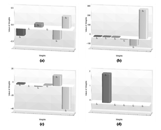
The proposed methodology EHPM accompanied by an efficient and powerful optimization technique is applied to the nonlinear problems defined above. The fitness function derived in the form (18) for the nonlinear problems (26), (28), (30) and (32) are optimized using the FA. The optimal weights achieved by the implementation of the developed technique at \alpha = 1, n = 5 and x \in \left[{0, 1} \right] yielding a fitness value 3.177187 \times {10^{ - 17}}, 4.316209 \times {10^{ - 12}}, and 1.43145 \times {10^{ - 17}} for the test problems 1–4 are displayed in Figure 2, respectively. The numerical results accomplished by the utilization of these optimal weights for the respective test problems are presented in Tables 1–4. Comparative study is conducted by comparing the EHPM computed results with the respective exact solution and the results attained by ABMA with the step size \bar h = 0.001 and \bar K = 1000, 10 term approximate solution by MHPM, the APSO computed results (for 800 iterations and swarm size equal to 40) and the seventh term approximate solutions obtained by the RPSM. To illustrate the reliability and accuracy of the suggested scheme EHPM the values of absolute error attained by the considering the exact solution as the reference solution of the respective problems 1–4 are also presented in Tables 1–4, respectively. It is observed that generally, the EHPM computed results for all the problems coincides the exact solution within five to ten decimal places of accuracy. The error norms {L_{rms}} and {L_\infty } acquired for the above problems by consuming the developed scheme EHPM for the computational domain x \in \left[{0, 1} \right] and at distinct values n are tabulated in Table 5. These error estimates presented in Table 5 ensures about the convergence and accuracy of the deliberated technique which is seen to be increased as n increases.
| t | {y_{EXACT}} | {y_{EHPM}} | {y_{ABMA}} | {y_{RPSM}} | {y_{MHPM}} | {y_{APSO}} | {P_{abs}} |
| 0.1 | 0.475021 | 0.475021 | 0.475021 | 0.475021 | 0.475021 | 0.474993 | 2.46866×10⁻⁹ |
| 0.2 | 0.450166 | 0.450166 | 0.450166 | 0.450166 | 0.450165 | 0.449984 | 8.11591×10⁻⁹ |
| 0.3 | 0.425557 | 0.425557 | 0.425557 | 0.425557 | 0.425552 | 0.425056 | 2.62871×10⁻⁹ |
| 0.4 | 0.401312 | 0.401312 | 0.401312 | 0.401312 | 0.401291 | 0.400332 | 6.47150×10⁻⁹ |
| 0.5 | 0.377541 | 0.377541 | 0.377541 | 0.377541 | 0.377476 | 0.375992 | 1.62494×10⁻⁹ |
| 0.6 | 0.354344 | 0.354344 | 0.354344 | 0.354344 | 0.354182 | 0.352276 | 6.16224×10⁻⁹ |
| 0.7 | 0.331812 | 0.331812 | 0.331812 | 0.331813 | 0.331462 | 0.329493 | 6.81599×10⁻¹⁰ |
| 0.8 | 0.310026 | 0.310026 | 0.310026 | 0.310028 | 0.309343 | 0.308033 | 6.05932×10⁻⁹ |
| 0.9 | 0.289050 | 0.289051 | 0.289051 | 0.289058 | 0.287820 | 0.288369 | 3.75236×10⁻⁹ |
| 1.0 | 0.268941 | 0.268941 | 0.268941 | 0.268961 | 0.266858 | 0.271073 | 4.53833×10⁻⁹ |
 DownLoad:
CSV
DownLoad:
CSV
| t | {y_{EXACT}} | {y_{EHPM}} | {y_{ABMA}} | {y_{RPSM}} | {y_{NHPM}} | {y_{APSO}} | {P_{abs}} |
| 0.1 | 0.110295 | 0.110323 | 0.110295 | 0.110295 | 0.110294 | 0.132598 | 2.79559×10⁻⁵ |
| 0.2 | 0.241976 | 0.241942 | 0.241976 | 0.241976 | 0.241965 | 0.275045 | 3.40483×10⁻⁵ |
| 0.3 | 0.395104 | 0.395107 | 0.395104 | 0.395089 | 0.395106 | 0.427310 | 2.56995×10⁻⁶ |
| 0.4 | 0.567812 | 0.567860 | 0.567811 | 0.56766 | 0.568115 | 0.589222 | 4.80912×10⁻⁵ |
| 0.5 | 0.756014 | 0.756031 | 0.756014 | 0.755134 | 0.757564 | 0.760469 | 1.68103×10⁻⁵ |
| 0.6 | 0.953566 | 0.953530 | 0.953565 | 0.949964 | 0.958259 | 0.940590 | 3.57596×10⁻⁵ |
| 0.7 | 1.152949 | 1.152943 | 1.152949 | 1.141423 | 1.163459 | 1.128970 | 5.97971×10⁻⁶ |
| 0.8 | 1.346364 | 1.346424 | 1.346363 | 1.315723 | 1.365240 | 1.324840 | 6.04658×10⁻⁵ |
| 0.9 | 1.526911 | 1.526896 | 1.526911 | 1.456545 | 1.554960 | 1.527270 | 1.51114×10⁻⁵ |
| 1.0 | 1.689498 | 1.689546 | 1.689498 | 1.546030 | 1.723810 | 1.735140 | 4.79364×10⁻⁵ |
DownLoad:
CSV
| t | {y_{EXACT}} | {y_{EHPM}} | {y_{ABMA}} | {y_{RPSM}} | {y_{MHPM}} | {y_{APSO}} | {P_{abs}} |
| 0.1 | 0.099668 | 0.099666 | 0.099668 | 0.099668 | 0.099668 | 0.103891 | 1.23113×10⁻⁶ |
| 0.2 | 0.197375 | 0.197378 | 0.197375 | 0.197375 | 0.197375 | 0.202649 | 2.55077×10⁻⁶ |
| 0.3 | 0.291313 | 0.291313 | 0.291313 | 0.291312 | 0.291312 | 0.295810 | 1.45452×10⁻⁷ |
| 0.4 | 0.379949 | 0.379946 | 0.379949 | 0.379944 | 0.379944 | 0.382931 | 2.41309×10⁻⁶ |
| 0.5 | 0.462117 | 0.462117 | 0.462117 | 0.462078 | 0.462078 | 0.463587 | 1.66903×10⁻⁷ |
| 0.6 | 0.537050 | 0.537052 | 0.537049 | 0.536857 | 0.536857 | 0.537380 | 2.46396×10⁻⁶ |
| 0.7 | 0.604368 | 0.604368 | 0.604368 | 0.603631 | 0.603631 | 0.603935 | 4.64338×10⁻⁷ |
| 0.8 | 0.664037 | 0.664034 | 0.664037 | 0.661706 | 0.661706 | 0.662905 | 2.81496×10⁻⁶ |
| 0.9 | 0.716298 | 0.716299 | 0.716298 | 0.709919 | 0.709919 | 0.713971 | 1.30183×10⁻⁶ |
| 1.0 | 0.761594 | 0.761592 | 0.761594 | 0.746032 | 0.746032 | 0.756838 | 2.22537×10⁻⁶ |
DownLoad:
CSV
| t | {y_{EXACT}} | {y_{EHPM}} | {y_{ABMA}} | {y_{MHPM}} | {y_{APSO}} | {P_{abs}} |
| 0.1 | 0.01 | 0.01 | 0.019966 | 0.001 | 0.012254 | 2.91364×10⁻¹³ |
| 0.2 | 0.04 | 0.04 | 0.079449 | 0.008 | 0.044342 | 1.58054×10⁻¹³ |
| 0.3 | 0.09 | 0.09 | 0.177089 | 0.027 | 0.096103 | 2.13080×10⁻¹³ |
| 0.4 | 0.16 | 0.16 | 0.310209 | 0.064 | 0.167389 | 4.90163×10⁻¹⁴ |
| 0.5 | 0.25 | 0.25 | 0.473957 | 0.125 | 0.258064 | 2.18325×10⁻¹³ |
| 0.6 | 0.36 | 0.36 | 0.659526 | 0.216 | 0.368016 | 8.49321×10⁻¹⁴ |
| 0.7 | 0.49 | 0.49 | 0.850389 | 0.343 | 0.497157 | 1.76026×10⁻¹³ |
| 0.8 | 0.64 | 0.64 | 1.014271 | 0.512 | 0.645426 | 1.66533×10⁻¹³ |
| 0.9 | 0.81 | 0.81 | 1.086366 | 0.729 | 0.812795 | 2.24820×10⁻¹³ |
| 1.0 | 1.00 | 1.00 | 0.938449 | 1.000 | 0.999274 | 3.39728×10⁻¹⁴ |
DownLoad:
CSV
| n | Test Problem 1 | Test Problem 2 | Test Problem 3 | Test Problem 4 | ||||
| {L_{rms}} | {L_\infty } | {L_{rms}} | {L_\infty } | {L_{rms}} | {L_\infty } | {L_{rms}} | {L_\infty } | |
| 5 | 4.82×10⁻⁹ | 8.11×10⁻⁹ | 3.46×10⁻⁵ | 6.04×10⁻⁵ | 1.86×10⁻⁶ | 2.81×10⁻⁶ | 1.79×10⁻¹³ | 2.91×10⁻¹³ |
| 4 | 1.98×10⁻⁷ | 2.63×10⁻⁷ | 1.67×10⁻⁴ | 2.63×10⁻⁴ | 1.78×10⁻⁵ | 2.36×10⁻⁵ | 1.73×10⁻¹⁴ | 3.25×10⁻¹⁴ |
| 3 | 1.86×10⁻⁶ | 3.04×10⁻⁶ | 1.12×10⁻³ | 2.01×10⁻³ | 3.33×10⁻⁵ | 6.10×10⁻⁵ | 6.49×10⁻⁹ | 1.13×10⁻⁸ |
| 2 | 2.94×10⁻⁵ | 5.27×10⁻⁵ | 3.51×10⁻³ | 6.39×10⁻³ | 1.03×10⁻³ | 1.76×10⁻³ | 5.17×10⁻⁹ | 8.62×10⁻⁹ |
DownLoad:
CSV
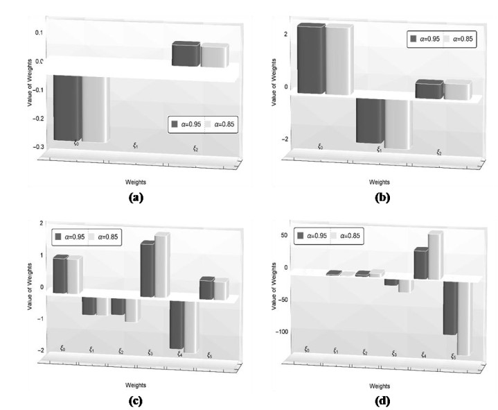
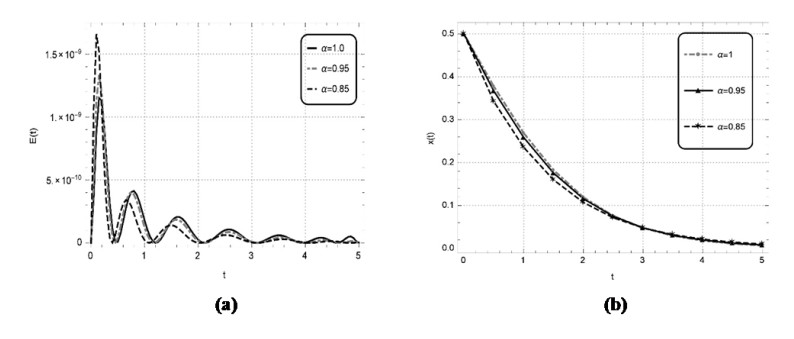
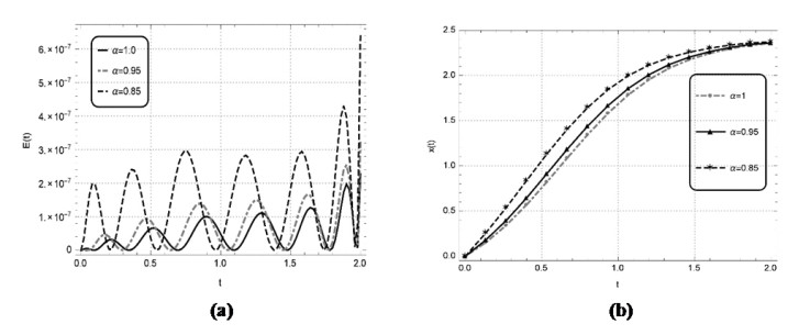
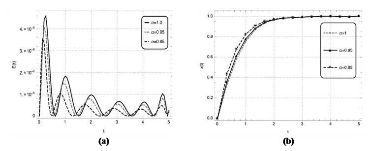
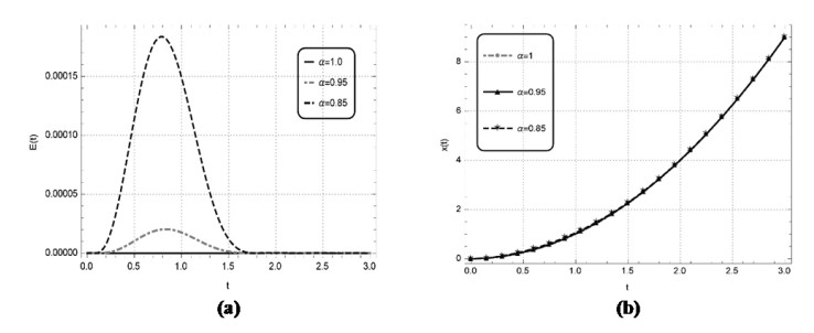
Numerical solutions of the above problems are also constructed by the discussed technique for the non-integer order. The solutions of the above nonlinear problems are attained by the learning of unknown weights in the derived fitness function at two distinct values of \alpha i.e., 0.95 and 0.85. The optimal weights achieved by the proposed scheme for the considered fractional values with n = 2 and x \in \left[{0, 1} \right] for problem 1, with n = 2 and x \in \left[{0, 4} \right] for problem 2, with n = 5 and x \in \left[{0, 5} \right] for problem 3 and with n = 5 and x \in \left[{0, 1} \right] for problem 4 are showcased in Figure 3, respectively. The results obtained by utilizing these real valued and bounded optimal weights for the respective problems 1–4 are presented in Tables 6–9, respectively. The results obtained by EHPM are compared with the available exact solution, MHPM computed results, seventh term approximate solutions obtained by the RPSM and the results attained by ABMA for the step \bar h = 0.001 and the values \bar K equal to 4000 and 5000 for the test problems 1–3, respectively. In problem 1 by taking smaller value n for a smaller domain \left[{0, 1} \right] the results achieved by the EHPM and the RPSM shows a constructive agreement with the results obtained by ABMA. While, by taking a smaller value n for a larger domain \left[{0, 4} \right] in problem 2, the RPSM is seen to diverge whereas, the solutions obtained by the EHPM remains convergent. By taking a larger value n for a larger domain \left[{0, 5} \right] in problem 3 the RPSM computed results diverges whereas, the results accomplished by the proposed scheme shows a constructive agreement with the results attained by ABMA. The values of absolute error achieved by EHPM for the problems 1–3 with the results attained by ABMA as the reference solution are also depicted in Tables 6–8. In problem 4 by taking a larger value of n for a smaller domain \left[{0, 1} \right] the EHPM computed results are compared with available exact solution and the results obtained by MHPM, with the values of absolute error tabulated in Table 9. Furthermore, the correctness and reliability of the suggested scheme is validated by the minimize fitness function and the related graphical solution attained at distinct values of \alpha = 1, 0.95, 0.85 for a lager span, that are portrayed in Figures 4a–7a and Figures 4b–7b for the problems 1–4, respectively. One can infer that the accuracy of the presented scheme can be further enhanced but at the cost of more computation.
| t | \alpha = 0.85 | \alpha = 0.95 | ||||||
| {y_{EHPM}} | {y_{ABMA}} | {y_{RPSM}} | {P_{abs}} | {y_{EHPM}} | {y_{ABMA}} | {y_{RPSM}} | {P_{abs}} | |
| 0.1 | 0.458464 | 0.462742 | 0.462742 | 4.27763×10⁻³ | 0.470459 | 0.471407 | 0.471407 | 9.4861×10⁻⁴ |
| 0.2 | 0.425630 | 0.433189 | 0.433189 | 7.55906×10⁻³ | 0.443171 | 0.444939 | 0.444939 | 1.76834×10⁻³ |
| 0.3 | 0.395869 | 0.406386 | 0.406387 | 1.05170×10⁻² | 0.416934 | 0.419474 | 0.419474 | 2.54007×10⁻³ |
| 0.4 | 0.368265 | 0.381546 | 0.381546 | 1.32809×10⁻² | 0.391583 | 0.394880 | 0.394880 | 3.29609×10⁻³ |
| 0.5 | 0.342440 | 0.358340 | 0.358340 | 1.58994×10⁻² | 0.367092 | 0.371144 | 0.371145 | 4.05246×10⁻³ |
| 0.6 | 0.318209 | 0.336593 | 0.336596 | 1.83840×10⁻² | 0.343479 | 0.348290 | 0.348291 | 4.81164×10⁻³ |
| 0.7 | 0.295471 | 0.316194 | 0.316201 | 2.07229×10⁻² | 0.320785 | 0.326348 | 0.326350 | 5.56302×10⁻³ |
| 0.8 | 0.274172 | 0.297059 | 0.297079 | 2.28877×10⁻² | 0.299065 | 0.305348 | 0.305353 | 6.28306×10⁻³ |
| 0.9 | 0.254283 | 0.279120 | 0.279167 | 2.48372×10⁻² | 0.278377 | 0.285313 | 0.285327 | 6.93573×10⁻³ |
| 1.0 | 0.235793 | 0.262314 | 0.262417 | 2.65208×10⁻² | 0.258786 | 0.266259 | 0.266294 | 7.47296×10⁻³ |
DownLoad:
CSV
| t | \alpha = 0.85 | \alpha = 0.95 | ||||||
| {y_{EHPM}} | {y_{ABMA}} | {y_{RPSM}} | {P_{abs}} | {y_{EHPM}} | {y_{ABMA}} | {y_{RPSM}} | {P_{abs}} | |
| 0.4 | 1.128780 | 0.772076 | 0.701892 | 3.56704×10⁻¹ | 0.951216 | 0.629409 | 0.609030 | 3.21808×10⁻¹ |
| 0.8 | 1.732609 | 1.534233 | 1.292070 | 1.98376×10⁻¹ | 1.582695 | 1.414490 | 1.339680 | 1.68205×10⁻¹ |
| 1.2 | 2.095352 | 1.965731 | -0.689702 | 1.29622×10⁻¹ | 1.999238 | 1.962805 | 1.116260 | 3.64331×10⁻² |
| 1.6 | 2.300624 | 2.159265 | -12.26610 | 1.41359×10⁻¹ | 2.252742 | 2.217871 | -1.984430 | 3.48714×10⁻² |
| 2.0 | 2.399864 | 2.248003 | -48.77540 | 1.51861×10⁻¹ | 2.384753 | 2.319886 | -9.224490 | 6.48668×10⁻² |
| 2.4 | 2.430901 | 2.293382 | -139.1670 | 1.37519×10⁻¹ | 2.431978 | 2.361076 | -17.66350 | 7.09018×10⁻² |
| 2.8 | 2.424109 | 2.319480 | -332.8130 | 1.04629×10⁻¹ | 2.428249 | 2.379249 | -13.99210 | 4.89996×10⁻² |
| 3.2 | 2.405166 | 2.336069 | -707.8470 | 6.90973×10⁻² | 2.405453 | 2.388335 | 34.79380 | 1.71183×10⁻² |
| 3.6 | 2.396527 | 2.347472 | -1381.040 | 4.90542×10⁻² | 2.394053 | 2.393514 | 194.3750 | 5.39429×10⁻⁴ |
| 4.0 | 2.418283 | 2.355791 | -2519.200 | 6.24925×10⁻² | 2.423411 | 2.396826 | 580.2210 | 2.65850×10⁻² |
DownLoad:
CSV
| t | \alpha = 0.85 | \alpha = 0.95 | ||||||
| {y_{EHPM}} | {y_{ABMA}} | {y_{RPSM}} | {P_{abs}} | {y_{EHPM}} | {y_{ABMA}} | {y_{RPSM}} | {P_{abs}} | |
| 0.5 | 0.571511 | 0.515900 | 0.481043 | 5.56103×10⁻² | 0.497222 | 0.481137 | 0.515392 | 1.60848×10⁻² |
| 1.0 | 0.824167 | 0.749435 | 0.731907 | 7.47319×10⁻² | 0.778543 | 0.758713 | 0.675115 | 1.98303×10⁻² |
| 1.5 | 0.933117 | 0.855319 | 0.263158 | 7.77975×10⁻² | 0.915829 | 0.888118 | -0.334334 | 2.77111×10⁻² |
| 2.0 | 0.972671 | 0.906026 | -4.400130 | 6.66455×10⁻² | 0.968915 | 0.943982 | -7.027070 | 2.49329×10⁻² |
| 2.5 | 0.986094 | 0.932703 | -25.95750 | 5.33910×10⁻² | 0.985180 | 0.968440 | -32.40280 | 1.67394×10⁻² |
| 3.0 | 0.993557 | 0.948165 | -97.30430 | 4.53923×10⁻² | 0.992469 | 0.979829 | -104.6460 | 1.26404×10⁻² |
| 3.5 | 0.999402 | 0.957932 | -288.1960 | 4.14707×10⁻² | 0.999263 | 0.985618 | -275.6610 | 1.36449×10⁻² |
| 4.0 | 1.000703 | 0.964556 | -728.4980 | 3.61731×10⁻² | 1.001750 | 0.988867 | -631.4190 | 1.28808×10⁻² |
| 4.5 | 0.997296 | 0.969315 | -1638.840 | 2.79813×10⁻² | 0.997197 | 0.990876 | -1304.100 | 6.32101×10⁻³ |
| 5.0 | 1.002409 | 0.972892 | -3369.480 | 2.95975×10⁻² | 1.003140 | 0.992229 | -2486.000 | 1.09120×10⁻² |
DownLoad:
CSV
| t | \alpha = 0.85 | \alpha = 0.95 | ||||||
| {y_{EHPM}} | {y_{EXACT}} | {y_{MHPM}} | {P_{abs}} | {y_{EHPM}} | {y_{EXACT}} | {y_{MHPM}} | {P_{abs}} | |
| 0.1 | 0.009336 | 0.01 | 0.001527 | 6.63272×10⁻⁴ | 0.009782 | 0.01 | 0.001150 | 2.17468×10⁻⁴ |
| 0.2 | 0.037202 | 0.04 | 0.011010 | 2.79761×10⁻³ | 0.039123 | 0.04 | 0.008892 | 8.76525×10⁻⁴ |
| 0.3 | 0.083691 | 0.09 | 0.034966 | 6.30802×10⁻³ | 0.087988 | 0.09 | 0.029411 | 2.01164×10⁻³ |
| 0.4 | 0.148502 | 0.16 | 0.079383 | 1.14971×10⁻² | 0.156347 | 0.16 | 0.068718 | 3.65298×10⁻³ |
| 0.5 | 0.231266 | 0.25 | 0.149941 | 1.87333×10⁻² | 0.244079 | 0.25 | 0.132726 | 5.92024×10⁻³ |
| 0.6 | 0.331497 | 0.36 | 0.251096 | 2.85027×10⁻² | 0.351006 | 0.36 | 0.227269 | 8.99314×10⁻³ |
| 0.7 | 0.448290 | 0.49 | 0.391189 | 4.17099×10⁻² | 0.476835 | 0.49 | 0.358125 | 1.31646×10⁻² |
| 0.8 | 0.579872 | 0.64 | 0.572354 | 6.01272×10⁻² | 0.621014 | 0.64 | 0.531020 | 1.89856×10⁻² |
| 0.9 | 0.723061 | 0.81 | 0.800662 | 8.69390×10⁻² | 0.782501 | 0.81 | 0.751641 | 2.74983×10⁻² |
| 1.0 | 0.872643 | 1.00 | 1.081081 | 1.27356×10⁻¹ | 0.959450 | 1.00 | 1.025641 | 4.05497×10⁻² |
DownLoad:
CSV
In this work, the nonlinear fractional differential equations with the fractional derivative and integral operators defined in the Caputo sense are successfully solved by a simple, accurate and reliable numerical technique. The designed methodology EHPM is an amalgamation of the classical homotopy perturbation technique with the modern bio-inspired metaheuristic technique. The FA which is based on the flashing behavior of fireflies fast track the procedure to determine the approximate solution of the considered nonlinear FDE. Some instructive examples were undertaken, with varying span and different number of terms in the assumed initial approximation to expound the potential ability of the proposed technique. The validity, applicability and computational efficiency of the EHPM is exposed by comparing the fast track outcomes achieved with the available exact solution and the solutions obtained by ABMA, APSO, MHPM and the RPSM. High accuracy and consistent convergence were ascertained by the accomplishment of the optimal values of the error norms. Thus, the contribution of the discussed scheme is abridged as follows:
● The expedite design methodology is well suited to solve the nonlinear FDE.
● The classical approach transformed the nonlinear FDE into an algebraic system which leads to a weighted series solution.
● Fitness function determined by a trivial fragment of the weighted series solution was optimized using the FA.
● Fast track outcomes were achieved by the modern optimization technique (FA).
● Numerical experiments ratified the correctness and reliability of the EHPM.
● Converging solutions were attained even for a larger computational domain.
● High accuracy and consistent convergence achieved by EHPM can be further enhanced by increasing the number of term in the initial approximation.
As the proposed design methodology exhibits a merger of classical idea with the modern optimizing metaheuristic technique, which offers promising converging results. One may utilize the recommended fusion to solve numerous other mathematical models or may even attempt to determine a new combination of modern optimization technique with the former traditional schemes.
The authors declare no conflict of interest.
| [1] | Submitted. |
| [2] |
B. Alvarez-Samaniego and D. Lannes, Large time existence for 3D water-waves and asymptotics, Invent. Math., 171 (2008), 485-541. doi: 10.1007/s00222-007-0088-4

|
| [3] |
B. Alvarez-Samaniego and D. Lannes, A Nash-Moser theorem for singular evolution equations. Application to the Serre and Green-Naghdi equations, Indiana Univ. Math. J., 57 (2008), 97-131. doi: 10.1512/iumj.2008.57.3200
|
| [4] |
E. Audusse, F. Bouchut, M.-O. Bristeau, R. Klein and B. Perthame, A fast and stable well-balanced scheme with hydrostatic reconstruction for Shallow Water flows, SIAM J. Sci. Comput., 25 (2004), 2050-2065. doi: 10.1137/S1064827503431090
|
| [5] | URL http://hal.inria.fr/hal-01063577, (Submitted) http://hal.inria.fr/hal-01063577/PDF/kin_hydrost.pdf. |
| [6] |
J.-L. Bona, T.-B. Benjamin and J.-J. Mahony, Model equations for long waves in nonlinear dispersive systems, Philos. Trans. Royal Soc. London Series A, 272 (1972), 47-78. doi: 10.1098/rsta.1972.0032
|
| [7] |
P. Bonneton, E. Barthelemy, F. Chazel, R. Cienfuegos, D. Lannes, F. Marche and M. Tissier, Recent advances in Serre-Green Naghdi modelling for wave transformation, breaking and runup processes, European Journal of Mechanics - B/Fluids, 30 (2011), 589-597, URL http://www.sciencedirect.com/science/article/pii/S0997754611000185, Special Issue: Nearshore Hydrodynamics. doi: 10.1016/j.euromechflu.2011.02.005
|
| [8] | F. Bouchut, An introduction to finite volume methods for hyperbolic conservation laws, ESAIM Proc., 15 (2005), 1-17. |
| [9] |
F. Bouchut, Nonlinear Stability of Finite Volume Methods for Hyperbolic Conservation Laws and Well-Balanced Schemes for Sources, Birkhäuser, 2004. doi: 10.1007/b93802
|
| [10] | F. Brezzi, On the existence, uniqueness and approximation of saddle-point problems arising from Lagrangian multipliers, Rev. Française Automat. Informat. Recherche Opérationnelle Sér. Rouge, 8 (1974), 129-151. |
| [11] | M.-O. Bristeau and B. Coussin, Boundary Conditions for the Shallow Water Equations Solved by Kinetic Schemes, Rapport de recherche RR-4282, INRIA, 2001, URL http://hal.inria.fr/inria-00072305, Projet M3N. |
| [12] |
M.-O. Bristeau, N. Goutal and J. Sainte-Marie, Numerical simulations of a non-hydrostatic Shallow Water model, Computers & Fluids, 47 (2011), 51-64. doi: 10.1016/j.compfluid.2011.02.013
|
| [13] |
M. O. Bristeau, A. Mangeney, J. Sainte-Marie and N. Seguin, An energy-consistent depth-averaged Euler system: Derivation and properties, Discrete Contin. Dyn. Syst. Ser. B, 20 (2015), 961-988, URL http://aimsciences.org/journals/displayArticlesnew.jsp?paperID=10801. doi: 10.3934/dcdsb.2015.20.961
|
| [14] |
M.-O. Bristeau and J. Sainte-Marie, Derivation of a non-hydrostatic shallow water model; Comparison with Saint-Venant and Boussinesq systems, Discrete Contin. Dyn. Syst. Ser. B, 10 (2008), 733-759. doi: 10.3934/dcdsb.2008.10.733
|
| [15] |
R. Camassa, D. Holm and J. Hyman, A new integrable shallow water equation, Adv. Appl. Math., 31 (1994), 1-33. doi: 10.1016/S0065-2156(08)70254-0
|
| [16] |
F. Chazel, D. Lannes and F. Marche, Numerical simulation of strongly nonlinear and dispersive waves using a Green-Naghdi model, J. Sci. Comput., 48 (2011), 105-116. doi: 10.1007/s10915-010-9395-9
|
| [17] |
A. J. Chorin, Numerical solution of the Navier-Stokes equations, Math. Comp., 22 (1968), 745-762. doi: 10.1090/S0025-5718-1968-0242392-2
|
| [18] |
M.-W. Dingemans, Wave Propagation Over Uneven Bottoms, Advanced Series on Ocean Engineering - World Scientific, 1997. doi: 10.1142/9789812796042
|
| [19] | M. Dingemans, Comparison of Computations with Boussinesq-like Models and Laboratory Measurements, Technical Report H1684-12, AST G8M Coastal Morphodybamics Research Programme, 1994. |
| [20] |
A. Duran and F. Marche, Discontinuous-Galerkin discretization of a new class of Green-Naghdi equations, Communications in Computational Physics, 17 (2015), 721-760, URL https://hal.archives-ouvertes.fr/hal-00980826. doi: 10.4208/cicp.150414.101014a
|
| [21] |
W. E and J.-G. Liu, Projection method I: Convergence and numerical boundary layers, SIAM J. Numer. Anal., 32 (1995), 1017-1057. doi: 10.1137/0732047
|
| [22] |
A. Ern and S. Meunier, A posteriori error analysis of euler-galerkin approximations to coupled elliptic-parabolic problems, ESAIM Math. Model. Numer. Anal., 43 (2009), 353-375, URL http://journals.cambridge.org/abstract\_S0764583X05000166. doi: 10.1051/m2an:2008048
|
| [23] |
E. Godlewski and P.-A. Raviart, Numerical Approximations of Hyperbolic Systems of Conservation Laws, Applied Mathematical Sciences, vol. 118, Springer, New York, 1996. doi: 10.1007/978-1-4612-0713-9
|
| [24] |
A. Green and P. Naghdi, A derivation of equations for wave propagation in water of variable depth, J. Fluid Mech., 78 (1976), 237-246. doi: 10.1017/S0022112076002425
|
| [25] | First Int. Conf. on Comput. Methods in Flow Analysis, Okayama University, Japan. |
| [26] | J.-L. Guermond, Some implementations of projection methods for Navier-Stokes equations, ESAIM: Mathematical Modelling and Numerical Analysis, 30 (1996), 637-667, URL http://eudml.org/doc/193818. |
| [27] |
J.-L. Guermond and J. Shen, On the error estimates for the rotational pressure-correction projection methods, Math. Comput., 73 (2004), 1719-1737, URL http://dblp.uni-trier.de/db/journals/moc/moc73.html#GuermondS04. doi: 10.1090/S0025-5718-03-01621-1
|
| [28] |
H. Johnston and J.-G. Liu, Accurate, stable and efficient Navier-Stokes solvers based on explicit treatment of the pressure term, Journal of Computational Physics, 199 (2004), 221-259, URL http://www.sciencedirect.com/science/article/pii/S002199910400083X. doi: 10.1016/j.jcp.2004.02.009
|
| [29] |
D. Lannes and P. Bonneton, Derivation of asymptotic two-dimensional time-dependent equations for surface water wave propagation, Physics of Fluids, 21 (2009), 016601. doi: 10.1063/1.3053183
|
| [30] |
O. Le Métayer, S. Gavrilyuk and S. Hank, A numerical scheme for the Green-Naghdi model, J. Comput. Phys., 229 (2010), 2034-2045. doi: 10.1016/j.jcp.2009.11.021
|
| [31] |
R.-J. LeVeque, Finite Volume Methods for Hyperbolic Problems, Cambridge University Press, 2002. doi: 10.1017/CBO9780511791253
|
| [32] |
O. Nwogu, Alternative form of Boussinesq equations for nearshore wave propagation, Journal of Waterway, Port, Coastal and Ocean Engineering, ASCE, 119 (1993), 618-638. doi: 10.1061/(ASCE)0733-950X(1993)119:6(618)
|
| [33] |
D. Peregrine, Long waves on a beach, J. Fluid Mech., 27 (1967), 815-827. doi: 10.1017/S0022112067002605
|
| [34] | O. Pironneau, Méthodes Des Éléments Finis Pour Les Fluides., Masson, 1988. |
| [35] |
R. Rannacher, On Chorin's projection method for the incompressible Navier-Stokes equations, in The Navier-Stokes Equations II - Theory and Numerical Methods (eds. G. Heywood John, K. Masuda, R. Rautmann and A. Solonnikov Vsevolod), vol. 1530 of Lecture Notes in Mathematics, Springer Berlin Heidelberg, 1992, 167-183, URL http://dx.doi.org/10.1007/BFb0090341. doi: 10.1007/BFb0090341
|
| [36] | 11th AIAA Computational Fluid Dynamic Conference, Orlando, FL, USA. |
| [37] |
J. Shen, On error estimates of the penalty method for unsteady Navier-Stokes equations, SIAM J. Numer. Anal., 32 (1995), 386-403. doi: 10.1137/0732016
|
| [38] |
W. C. Thacker, Some exact solutions to the non-linear shallow water wave equations, J. Fluid Mech., 107 (1981), 499-508. doi: 10.1017/S0022112081001882
|
| 1. | Najeeb Alam Khan, Samreen Ahmed, Oyoon Abdul Razzaq, Ahmad Kamil Mahmood, Exploring fractional order 2‐D Helmholtz equation using finite difference scheme through the bat optimization algorithm, 2021, 0170-4214, 10.1002/mma.7271 | |
| 2. | Najeeb Alam Khan, Samreen Ahmed, Finite Difference Method with Metaheuristic Orientation for Exploration of Time Fractional Partial Differential Equations, 2021, 7, 2349-5103, 10.1007/s40819-021-01061-y | |
| 3. | Moa’ath N. Oqielat, Tareq Eriqat, Zeyad Al-Zhour, Osama Ogilat, Ahmad El-Ajou, Ishak Hashim, Construction of fractional series solutions to nonlinear fractional reaction–diffusion for bacteria growth model via Laplace residual power series method, 2022, 2195-268X, 10.1007/s40435-022-01001-8 | |
| 4. | Mohamed A. Abd El Salam, Mohamed A. Ramadan, Mahmoud A. Nassar, Praveen Agarwal, Yu-Ming Chu, Matrix computational collocation approach based on rational Chebyshev functions for nonlinear differential equations, 2021, 2021, 1687-1847, 10.1186/s13662-021-03481-y | |
| 5. | Ahmed B. Khoshaim, Muhammad Naeem, Ali Akgul, Nejib Ghanmi, Shamsullah Zaland, Lakhdar Ragoub, Novel Analysis of Fractional-Order Fifth-Order Korteweg–de Vries Equations, 2022, 2022, 2314-4785, 1, 10.1155/2022/1883268 |
Nora Aïssiouene, Marie-Odile Bristeau, Edwige Godlewski, Jacques Sainte-Marie. A combined finite volume - finite element scheme for a dispersive shallow water system[J]. Networks and Heterogeneous Media, 2016, 11(1): 1-27. doi: 10.3934/nhm.2016.11.1

| t | {y_{EXACT}} | {y_{EHPM}} | {y_{ABMA}} | {y_{RPSM}} | {y_{MHPM}} | {y_{APSO}} | {P_{abs}} |
| 0.1 | 0.475021 | 0.475021 | 0.475021 | 0.475021 | 0.475021 | 0.474993 | 2.46866×10⁻⁹ |
| 0.2 | 0.450166 | 0.450166 | 0.450166 | 0.450166 | 0.450165 | 0.449984 | 8.11591×10⁻⁹ |
| 0.3 | 0.425557 | 0.425557 | 0.425557 | 0.425557 | 0.425552 | 0.425056 | 2.62871×10⁻⁹ |
| 0.4 | 0.401312 | 0.401312 | 0.401312 | 0.401312 | 0.401291 | 0.400332 | 6.47150×10⁻⁹ |
| 0.5 | 0.377541 | 0.377541 | 0.377541 | 0.377541 | 0.377476 | 0.375992 | 1.62494×10⁻⁹ |
| 0.6 | 0.354344 | 0.354344 | 0.354344 | 0.354344 | 0.354182 | 0.352276 | 6.16224×10⁻⁹ |
| 0.7 | 0.331812 | 0.331812 | 0.331812 | 0.331813 | 0.331462 | 0.329493 | 6.81599×10⁻¹⁰ |
| 0.8 | 0.310026 | 0.310026 | 0.310026 | 0.310028 | 0.309343 | 0.308033 | 6.05932×10⁻⁹ |
| 0.9 | 0.289050 | 0.289051 | 0.289051 | 0.289058 | 0.287820 | 0.288369 | 3.75236×10⁻⁹ |
| 1.0 | 0.268941 | 0.268941 | 0.268941 | 0.268961 | 0.266858 | 0.271073 | 4.53833×10⁻⁹ |
DownLoad:
CSV
| t | {y_{EXACT}} | {y_{EHPM}} | {y_{ABMA}} | {y_{RPSM}} | {y_{NHPM}} | {y_{APSO}} | {P_{abs}} |
| 0.1 | 0.110295 | 0.110323 | 0.110295 | 0.110295 | 0.110294 | 0.132598 | 2.79559×10⁻⁵ |
| 0.2 | 0.241976 | 0.241942 | 0.241976 | 0.241976 | 0.241965 | 0.275045 | 3.40483×10⁻⁵ |
| 0.3 | 0.395104 | 0.395107 | 0.395104 | 0.395089 | 0.395106 | 0.427310 | 2.56995×10⁻⁶ |
| 0.4 | 0.567812 | 0.567860 | 0.567811 | 0.56766 | 0.568115 | 0.589222 | 4.80912×10⁻⁵ |
| 0.5 | 0.756014 | 0.756031 | 0.756014 | 0.755134 | 0.757564 | 0.760469 | 1.68103×10⁻⁵ |
| 0.6 | 0.953566 | 0.953530 | 0.953565 | 0.949964 | 0.958259 | 0.940590 | 3.57596×10⁻⁵ |
| 0.7 | 1.152949 | 1.152943 | 1.152949 | 1.141423 | 1.163459 | 1.128970 | 5.97971×10⁻⁶ |
| 0.8 | 1.346364 | 1.346424 | 1.346363 | 1.315723 | 1.365240 | 1.324840 | 6.04658×10⁻⁵ |
| 0.9 | 1.526911 | 1.526896 | 1.526911 | 1.456545 | 1.554960 | 1.527270 | 1.51114×10⁻⁵ |
| 1.0 | 1.689498 | 1.689546 | 1.689498 | 1.546030 | 1.723810 | 1.735140 | 4.79364×10⁻⁵ |
DownLoad:
CSV
| t | {y_{EXACT}} | {y_{EHPM}} | {y_{ABMA}} | {y_{RPSM}} | {y_{MHPM}} | {y_{APSO}} | {P_{abs}} |
| 0.1 | 0.099668 | 0.099666 | 0.099668 | 0.099668 | 0.099668 | 0.103891 | 1.23113×10⁻⁶ |
| 0.2 | 0.197375 | 0.197378 | 0.197375 | 0.197375 | 0.197375 | 0.202649 | 2.55077×10⁻⁶ |
| 0.3 | 0.291313 | 0.291313 | 0.291313 | 0.291312 | 0.291312 | 0.295810 | 1.45452×10⁻⁷ |
| 0.4 | 0.379949 | 0.379946 | 0.379949 | 0.379944 | 0.379944 | 0.382931 | 2.41309×10⁻⁶ |
| 0.5 | 0.462117 | 0.462117 | 0.462117 | 0.462078 | 0.462078 | 0.463587 | 1.66903×10⁻⁷ |
| 0.6 | 0.537050 | 0.537052 | 0.537049 | 0.536857 | 0.536857 | 0.537380 | 2.46396×10⁻⁶ |
| 0.7 | 0.604368 | 0.604368 | 0.604368 | 0.603631 | 0.603631 | 0.603935 | 4.64338×10⁻⁷ |
| 0.8 | 0.664037 | 0.664034 | 0.664037 | 0.661706 | 0.661706 | 0.662905 | 2.81496×10⁻⁶ |
| 0.9 | 0.716298 | 0.716299 | 0.716298 | 0.709919 | 0.709919 | 0.713971 | 1.30183×10⁻⁶ |
| 1.0 | 0.761594 | 0.761592 | 0.761594 | 0.746032 | 0.746032 | 0.756838 | 2.22537×10⁻⁶ |
DownLoad:
CSV
| t | {y_{EXACT}} | {y_{EHPM}} | {y_{ABMA}} | {y_{MHPM}} | {y_{APSO}} | {P_{abs}} |
| 0.1 | 0.01 | 0.01 | 0.019966 | 0.001 | 0.012254 | 2.91364×10⁻¹³ |
| 0.2 | 0.04 | 0.04 | 0.079449 | 0.008 | 0.044342 | 1.58054×10⁻¹³ |
| 0.3 | 0.09 | 0.09 | 0.177089 | 0.027 | 0.096103 | 2.13080×10⁻¹³ |
| 0.4 | 0.16 | 0.16 | 0.310209 | 0.064 | 0.167389 | 4.90163×10⁻¹⁴ |
| 0.5 | 0.25 | 0.25 | 0.473957 | 0.125 | 0.258064 | 2.18325×10⁻¹³ |
| 0.6 | 0.36 | 0.36 | 0.659526 | 0.216 | 0.368016 | 8.49321×10⁻¹⁴ |
| 0.7 | 0.49 | 0.49 | 0.850389 | 0.343 | 0.497157 | 1.76026×10⁻¹³ |
| 0.8 | 0.64 | 0.64 | 1.014271 | 0.512 | 0.645426 | 1.66533×10⁻¹³ |
| 0.9 | 0.81 | 0.81 | 1.086366 | 0.729 | 0.812795 | 2.24820×10⁻¹³ |
| 1.0 | 1.00 | 1.00 | 0.938449 | 1.000 | 0.999274 | 3.39728×10⁻¹⁴ |
DownLoad:
CSV
| n | Test Problem 1 | Test Problem 2 | Test Problem 3 | Test Problem 4 | ||||
| {L_{rms}} | {L_\infty } | {L_{rms}} | {L_\infty } | {L_{rms}} | {L_\infty } | {L_{rms}} | {L_\infty } | |
| 5 | 4.82×10⁻⁹ | 8.11×10⁻⁹ | 3.46×10⁻⁵ | 6.04×10⁻⁵ | 1.86×10⁻⁶ | 2.81×10⁻⁶ | 1.79×10⁻¹³ | 2.91×10⁻¹³ |
| 4 | 1.98×10⁻⁷ | 2.63×10⁻⁷ | 1.67×10⁻⁴ | 2.63×10⁻⁴ | 1.78×10⁻⁵ | 2.36×10⁻⁵ | 1.73×10⁻¹⁴ | 3.25×10⁻¹⁴ |
| 3 | 1.86×10⁻⁶ | 3.04×10⁻⁶ | 1.12×10⁻³ | 2.01×10⁻³ | 3.33×10⁻⁵ | 6.10×10⁻⁵ | 6.49×10⁻⁹ | 1.13×10⁻⁸ |
| 2 | 2.94×10⁻⁵ | 5.27×10⁻⁵ | 3.51×10⁻³ | 6.39×10⁻³ | 1.03×10⁻³ | 1.76×10⁻³ | 5.17×10⁻⁹ | 8.62×10⁻⁹ |
DownLoad:
CSV
| t | \alpha = 0.85 | \alpha = 0.95 | ||||||
| {y_{EHPM}} | {y_{ABMA}} | {y_{RPSM}} | {P_{abs}} | {y_{EHPM}} | {y_{ABMA}} | {y_{RPSM}} | {P_{abs}} | |
| 0.1 | 0.458464 | 0.462742 | 0.462742 | 4.27763×10⁻³ | 0.470459 | 0.471407 | 0.471407 | 9.4861×10⁻⁴ |
| 0.2 | 0.425630 | 0.433189 | 0.433189 | 7.55906×10⁻³ | 0.443171 | 0.444939 | 0.444939 | 1.76834×10⁻³ |
| 0.3 | 0.395869 | 0.406386 | 0.406387 | 1.05170×10⁻² | 0.416934 | 0.419474 | 0.419474 | 2.54007×10⁻³ |
| 0.4 | 0.368265 | 0.381546 | 0.381546 | 1.32809×10⁻² | 0.391583 | 0.394880 | 0.394880 | 3.29609×10⁻³ |
| 0.5 | 0.342440 | 0.358340 | 0.358340 | 1.58994×10⁻² | 0.367092 | 0.371144 | 0.371145 | 4.05246×10⁻³ |
| 0.6 | 0.318209 | 0.336593 | 0.336596 | 1.83840×10⁻² | 0.343479 | 0.348290 | 0.348291 | 4.81164×10⁻³ |
| 0.7 | 0.295471 | 0.316194 | 0.316201 | 2.07229×10⁻² | 0.320785 | 0.326348 | 0.326350 | 5.56302×10⁻³ |
| 0.8 | 0.274172 | 0.297059 | 0.297079 | 2.28877×10⁻² | 0.299065 | 0.305348 | 0.305353 | 6.28306×10⁻³ |
| 0.9 | 0.254283 | 0.279120 | 0.279167 | 2.48372×10⁻² | 0.278377 | 0.285313 | 0.285327 | 6.93573×10⁻³ |
| 1.0 | 0.235793 | 0.262314 | 0.262417 | 2.65208×10⁻² | 0.258786 | 0.266259 | 0.266294 | 7.47296×10⁻³ |
DownLoad:
CSV
| t | \alpha = 0.85 | \alpha = 0.95 | ||||||
| {y_{EHPM}} | {y_{ABMA}} | {y_{RPSM}} | {P_{abs}} | {y_{EHPM}} | {y_{ABMA}} | {y_{RPSM}} | {P_{abs}} | |
| 0.4 | 1.128780 | 0.772076 | 0.701892 | 3.56704×10⁻¹ | 0.951216 | 0.629409 | 0.609030 | 3.21808×10⁻¹ |
| 0.8 | 1.732609 | 1.534233 | 1.292070 | 1.98376×10⁻¹ | 1.582695 | 1.414490 | 1.339680 | 1.68205×10⁻¹ |
| 1.2 | 2.095352 | 1.965731 | -0.689702 | 1.29622×10⁻¹ | 1.999238 | 1.962805 | 1.116260 | 3.64331×10⁻² |
| 1.6 | 2.300624 | 2.159265 | -12.26610 | 1.41359×10⁻¹ | 2.252742 | 2.217871 | -1.984430 | 3.48714×10⁻² |
| 2.0 | 2.399864 | 2.248003 | -48.77540 | 1.51861×10⁻¹ | 2.384753 | 2.319886 | -9.224490 | 6.48668×10⁻² |
| 2.4 | 2.430901 | 2.293382 | -139.1670 | 1.37519×10⁻¹ | 2.431978 | 2.361076 | -17.66350 | 7.09018×10⁻² |
| 2.8 | 2.424109 | 2.319480 | -332.8130 | 1.04629×10⁻¹ | 2.428249 | 2.379249 | -13.99210 | 4.89996×10⁻² |
| 3.2 | 2.405166 | 2.336069 | -707.8470 | 6.90973×10⁻² | 2.405453 | 2.388335 | 34.79380 | 1.71183×10⁻² |
| 3.6 | 2.396527 | 2.347472 | -1381.040 | 4.90542×10⁻² | 2.394053 | 2.393514 | 194.3750 | 5.39429×10⁻⁴ |
| 4.0 | 2.418283 | 2.355791 | -2519.200 | 6.24925×10⁻² | 2.423411 | 2.396826 | 580.2210 | 2.65850×10⁻² |
DownLoad:
CSV
| t | \alpha = 0.85 | \alpha = 0.95 | ||||||
| {y_{EHPM}} | {y_{ABMA}} | {y_{RPSM}} | {P_{abs}} | {y_{EHPM}} | {y_{ABMA}} | {y_{RPSM}} | {P_{abs}} | |
| 0.5 | 0.571511 | 0.515900 | 0.481043 | 5.56103×10⁻² | 0.497222 | 0.481137 | 0.515392 | 1.60848×10⁻² |
| 1.0 | 0.824167 | 0.749435 | 0.731907 | 7.47319×10⁻² | 0.778543 | 0.758713 | 0.675115 | 1.98303×10⁻² |
| 1.5 | 0.933117 | 0.855319 | 0.263158 | 7.77975×10⁻² | 0.915829 | 0.888118 | -0.334334 | 2.77111×10⁻² |
| 2.0 | 0.972671 | 0.906026 | -4.400130 | 6.66455×10⁻² | 0.968915 | 0.943982 | -7.027070 | 2.49329×10⁻² |
| 2.5 | 0.986094 | 0.932703 | -25.95750 | 5.33910×10⁻² | 0.985180 | 0.968440 | -32.40280 | 1.67394×10⁻² |
| 3.0 | 0.993557 | 0.948165 | -97.30430 | 4.53923×10⁻² | 0.992469 | 0.979829 | -104.6460 | 1.26404×10⁻² |
| 3.5 | 0.999402 | 0.957932 | -288.1960 | 4.14707×10⁻² | 0.999263 | 0.985618 | -275.6610 | 1.36449×10⁻² |
| 4.0 | 1.000703 | 0.964556 | -728.4980 | 3.61731×10⁻² | 1.001750 | 0.988867 | -631.4190 | 1.28808×10⁻² |
| 4.5 | 0.997296 | 0.969315 | -1638.840 | 2.79813×10⁻² | 0.997197 | 0.990876 | -1304.100 | 6.32101×10⁻³ |
| 5.0 | 1.002409 | 0.972892 | -3369.480 | 2.95975×10⁻² | 1.003140 | 0.992229 | -2486.000 | 1.09120×10⁻² |
DownLoad:
CSV
| t | \alpha = 0.85 | \alpha = 0.95 | ||||||
| {y_{EHPM}} | {y_{EXACT}} | {y_{MHPM}} | {P_{abs}} | {y_{EHPM}} | {y_{EXACT}} | {y_{MHPM}} | {P_{abs}} | |
| 0.1 | 0.009336 | 0.01 | 0.001527 | 6.63272×10⁻⁴ | 0.009782 | 0.01 | 0.001150 | 2.17468×10⁻⁴ |
| 0.2 | 0.037202 | 0.04 | 0.011010 | 2.79761×10⁻³ | 0.039123 | 0.04 | 0.008892 | 8.76525×10⁻⁴ |
| 0.3 | 0.083691 | 0.09 | 0.034966 | 6.30802×10⁻³ | 0.087988 | 0.09 | 0.029411 | 2.01164×10⁻³ |
| 0.4 | 0.148502 | 0.16 | 0.079383 | 1.14971×10⁻² | 0.156347 | 0.16 | 0.068718 | 3.65298×10⁻³ |
| 0.5 | 0.231266 | 0.25 | 0.149941 | 1.87333×10⁻² | 0.244079 | 0.25 | 0.132726 | 5.92024×10⁻³ |
| 0.6 | 0.331497 | 0.36 | 0.251096 | 2.85027×10⁻² | 0.351006 | 0.36 | 0.227269 | 8.99314×10⁻³ |
| 0.7 | 0.448290 | 0.49 | 0.391189 | 4.17099×10⁻² | 0.476835 | 0.49 | 0.358125 | 1.31646×10⁻² |
| 0.8 | 0.579872 | 0.64 | 0.572354 | 6.01272×10⁻² | 0.621014 | 0.64 | 0.531020 | 1.89856×10⁻² |
| 0.9 | 0.723061 | 0.81 | 0.800662 | 8.69390×10⁻² | 0.782501 | 0.81 | 0.751641 | 2.74983×10⁻² |
| 1.0 | 0.872643 | 1.00 | 1.081081 | 1.27356×10⁻¹ | 0.959450 | 1.00 | 1.025641 | 4.05497×10⁻² |
DownLoad:
CSV
| t | {y_{EXACT}} | {y_{EHPM}} | {y_{ABMA}} | {y_{RPSM}} | {y_{MHPM}} | {y_{APSO}} | {P_{abs}} |
| 0.1 | 0.475021 | 0.475021 | 0.475021 | 0.475021 | 0.475021 | 0.474993 | 2.46866×10⁻⁹ |
| 0.2 | 0.450166 | 0.450166 | 0.450166 | 0.450166 | 0.450165 | 0.449984 | 8.11591×10⁻⁹ |
| 0.3 | 0.425557 | 0.425557 | 0.425557 | 0.425557 | 0.425552 | 0.425056 | 2.62871×10⁻⁹ |
| 0.4 | 0.401312 | 0.401312 | 0.401312 | 0.401312 | 0.401291 | 0.400332 | 6.47150×10⁻⁹ |
| 0.5 | 0.377541 | 0.377541 | 0.377541 | 0.377541 | 0.377476 | 0.375992 | 1.62494×10⁻⁹ |
| 0.6 | 0.354344 | 0.354344 | 0.354344 | 0.354344 | 0.354182 | 0.352276 | 6.16224×10⁻⁹ |
| 0.7 | 0.331812 | 0.331812 | 0.331812 | 0.331813 | 0.331462 | 0.329493 | 6.81599×10⁻¹⁰ |
| 0.8 | 0.310026 | 0.310026 | 0.310026 | 0.310028 | 0.309343 | 0.308033 | 6.05932×10⁻⁹ |
| 0.9 | 0.289050 | 0.289051 | 0.289051 | 0.289058 | 0.287820 | 0.288369 | 3.75236×10⁻⁹ |
| 1.0 | 0.268941 | 0.268941 | 0.268941 | 0.268961 | 0.266858 | 0.271073 | 4.53833×10⁻⁹ |
| t | {y_{EXACT}} | {y_{EHPM}} | {y_{ABMA}} | {y_{RPSM}} | {y_{NHPM}} | {y_{APSO}} | {P_{abs}} |
| 0.1 | 0.110295 | 0.110323 | 0.110295 | 0.110295 | 0.110294 | 0.132598 | 2.79559×10⁻⁵ |
| 0.2 | 0.241976 | 0.241942 | 0.241976 | 0.241976 | 0.241965 | 0.275045 | 3.40483×10⁻⁵ |
| 0.3 | 0.395104 | 0.395107 | 0.395104 | 0.395089 | 0.395106 | 0.427310 | 2.56995×10⁻⁶ |
| 0.4 | 0.567812 | 0.567860 | 0.567811 | 0.56766 | 0.568115 | 0.589222 | 4.80912×10⁻⁵ |
| 0.5 | 0.756014 | 0.756031 | 0.756014 | 0.755134 | 0.757564 | 0.760469 | 1.68103×10⁻⁵ |
| 0.6 | 0.953566 | 0.953530 | 0.953565 | 0.949964 | 0.958259 | 0.940590 | 3.57596×10⁻⁵ |
| 0.7 | 1.152949 | 1.152943 | 1.152949 | 1.141423 | 1.163459 | 1.128970 | 5.97971×10⁻⁶ |
| 0.8 | 1.346364 | 1.346424 | 1.346363 | 1.315723 | 1.365240 | 1.324840 | 6.04658×10⁻⁵ |
| 0.9 | 1.526911 | 1.526896 | 1.526911 | 1.456545 | 1.554960 | 1.527270 | 1.51114×10⁻⁵ |
| 1.0 | 1.689498 | 1.689546 | 1.689498 | 1.546030 | 1.723810 | 1.735140 | 4.79364×10⁻⁵ |
| t | {y_{EXACT}} | {y_{EHPM}} | {y_{ABMA}} | {y_{RPSM}} | {y_{MHPM}} | {y_{APSO}} | {P_{abs}} |
| 0.1 | 0.099668 | 0.099666 | 0.099668 | 0.099668 | 0.099668 | 0.103891 | 1.23113×10⁻⁶ |
| 0.2 | 0.197375 | 0.197378 | 0.197375 | 0.197375 | 0.197375 | 0.202649 | 2.55077×10⁻⁶ |
| 0.3 | 0.291313 | 0.291313 | 0.291313 | 0.291312 | 0.291312 | 0.295810 | 1.45452×10⁻⁷ |
| 0.4 | 0.379949 | 0.379946 | 0.379949 | 0.379944 | 0.379944 | 0.382931 | 2.41309×10⁻⁶ |
| 0.5 | 0.462117 | 0.462117 | 0.462117 | 0.462078 | 0.462078 | 0.463587 | 1.66903×10⁻⁷ |
| 0.6 | 0.537050 | 0.537052 | 0.537049 | 0.536857 | 0.536857 | 0.537380 | 2.46396×10⁻⁶ |
| 0.7 | 0.604368 | 0.604368 | 0.604368 | 0.603631 | 0.603631 | 0.603935 | 4.64338×10⁻⁷ |
| 0.8 | 0.664037 | 0.664034 | 0.664037 | 0.661706 | 0.661706 | 0.662905 | 2.81496×10⁻⁶ |
| 0.9 | 0.716298 | 0.716299 | 0.716298 | 0.709919 | 0.709919 | 0.713971 | 1.30183×10⁻⁶ |
| 1.0 | 0.761594 | 0.761592 | 0.761594 | 0.746032 | 0.746032 | 0.756838 | 2.22537×10⁻⁶ |
| t | {y_{EXACT}} | {y_{EHPM}} | {y_{ABMA}} | {y_{MHPM}} | {y_{APSO}} | {P_{abs}} |
| 0.1 | 0.01 | 0.01 | 0.019966 | 0.001 | 0.012254 | 2.91364×10⁻¹³ |
| 0.2 | 0.04 | 0.04 | 0.079449 | 0.008 | 0.044342 | 1.58054×10⁻¹³ |
| 0.3 | 0.09 | 0.09 | 0.177089 | 0.027 | 0.096103 | 2.13080×10⁻¹³ |
| 0.4 | 0.16 | 0.16 | 0.310209 | 0.064 | 0.167389 | 4.90163×10⁻¹⁴ |
| 0.5 | 0.25 | 0.25 | 0.473957 | 0.125 | 0.258064 | 2.18325×10⁻¹³ |
| 0.6 | 0.36 | 0.36 | 0.659526 | 0.216 | 0.368016 | 8.49321×10⁻¹⁴ |
| 0.7 | 0.49 | 0.49 | 0.850389 | 0.343 | 0.497157 | 1.76026×10⁻¹³ |
| 0.8 | 0.64 | 0.64 | 1.014271 | 0.512 | 0.645426 | 1.66533×10⁻¹³ |
| 0.9 | 0.81 | 0.81 | 1.086366 | 0.729 | 0.812795 | 2.24820×10⁻¹³ |
| 1.0 | 1.00 | 1.00 | 0.938449 | 1.000 | 0.999274 | 3.39728×10⁻¹⁴ |
| n | Test Problem 1 | Test Problem 2 | Test Problem 3 | Test Problem 4 | ||||
| {L_{rms}} | {L_\infty } | {L_{rms}} | {L_\infty } | {L_{rms}} | {L_\infty } | {L_{rms}} | {L_\infty } | |
| 5 | 4.82×10⁻⁹ | 8.11×10⁻⁹ | 3.46×10⁻⁵ | 6.04×10⁻⁵ | 1.86×10⁻⁶ | 2.81×10⁻⁶ | 1.79×10⁻¹³ | 2.91×10⁻¹³ |
| 4 | 1.98×10⁻⁷ | 2.63×10⁻⁷ | 1.67×10⁻⁴ | 2.63×10⁻⁴ | 1.78×10⁻⁵ | 2.36×10⁻⁵ | 1.73×10⁻¹⁴ | 3.25×10⁻¹⁴ |
| 3 | 1.86×10⁻⁶ | 3.04×10⁻⁶ | 1.12×10⁻³ | 2.01×10⁻³ | 3.33×10⁻⁵ | 6.10×10⁻⁵ | 6.49×10⁻⁹ | 1.13×10⁻⁸ |
| 2 | 2.94×10⁻⁵ | 5.27×10⁻⁵ | 3.51×10⁻³ | 6.39×10⁻³ | 1.03×10⁻³ | 1.76×10⁻³ | 5.17×10⁻⁹ | 8.62×10⁻⁹ |
| t | \alpha = 0.85 | \alpha = 0.95 | ||||||
| {y_{EHPM}} | {y_{ABMA}} | {y_{RPSM}} | {P_{abs}} | {y_{EHPM}} | {y_{ABMA}} | {y_{RPSM}} | {P_{abs}} | |
| 0.1 | 0.458464 | 0.462742 | 0.462742 | 4.27763×10⁻³ | 0.470459 | 0.471407 | 0.471407 | 9.4861×10⁻⁴ |
| 0.2 | 0.425630 | 0.433189 | 0.433189 | 7.55906×10⁻³ | 0.443171 | 0.444939 | 0.444939 | 1.76834×10⁻³ |
| 0.3 | 0.395869 | 0.406386 | 0.406387 | 1.05170×10⁻² | 0.416934 | 0.419474 | 0.419474 | 2.54007×10⁻³ |
| 0.4 | 0.368265 | 0.381546 | 0.381546 | 1.32809×10⁻² | 0.391583 | 0.394880 | 0.394880 | 3.29609×10⁻³ |
| 0.5 | 0.342440 | 0.358340 | 0.358340 | 1.58994×10⁻² | 0.367092 | 0.371144 | 0.371145 | 4.05246×10⁻³ |
| 0.6 | 0.318209 | 0.336593 | 0.336596 | 1.83840×10⁻² | 0.343479 | 0.348290 | 0.348291 | 4.81164×10⁻³ |
| 0.7 | 0.295471 | 0.316194 | 0.316201 | 2.07229×10⁻² | 0.320785 | 0.326348 | 0.326350 | 5.56302×10⁻³ |
| 0.8 | 0.274172 | 0.297059 | 0.297079 | 2.28877×10⁻² | 0.299065 | 0.305348 | 0.305353 | 6.28306×10⁻³ |
| 0.9 | 0.254283 | 0.279120 | 0.279167 | 2.48372×10⁻² | 0.278377 | 0.285313 | 0.285327 | 6.93573×10⁻³ |
| 1.0 | 0.235793 | 0.262314 | 0.262417 | 2.65208×10⁻² | 0.258786 | 0.266259 | 0.266294 | 7.47296×10⁻³ |
| t | \alpha = 0.85 | \alpha = 0.95 | ||||||
| {y_{EHPM}} | {y_{ABMA}} | {y_{RPSM}} | {P_{abs}} | {y_{EHPM}} | {y_{ABMA}} | {y_{RPSM}} | {P_{abs}} | |
| 0.4 | 1.128780 | 0.772076 | 0.701892 | 3.56704×10⁻¹ | 0.951216 | 0.629409 | 0.609030 | 3.21808×10⁻¹ |
| 0.8 | 1.732609 | 1.534233 | 1.292070 | 1.98376×10⁻¹ | 1.582695 | 1.414490 | 1.339680 | 1.68205×10⁻¹ |
| 1.2 | 2.095352 | 1.965731 | -0.689702 | 1.29622×10⁻¹ | 1.999238 | 1.962805 | 1.116260 | 3.64331×10⁻² |
| 1.6 | 2.300624 | 2.159265 | -12.26610 | 1.41359×10⁻¹ | 2.252742 | 2.217871 | -1.984430 | 3.48714×10⁻² |
| 2.0 | 2.399864 | 2.248003 | -48.77540 | 1.51861×10⁻¹ | 2.384753 | 2.319886 | -9.224490 | 6.48668×10⁻² |
| 2.4 | 2.430901 | 2.293382 | -139.1670 | 1.37519×10⁻¹ | 2.431978 | 2.361076 | -17.66350 | 7.09018×10⁻² |
| 2.8 | 2.424109 | 2.319480 | -332.8130 | 1.04629×10⁻¹ | 2.428249 | 2.379249 | -13.99210 | 4.89996×10⁻² |
| 3.2 | 2.405166 | 2.336069 | -707.8470 | 6.90973×10⁻² | 2.405453 | 2.388335 | 34.79380 | 1.71183×10⁻² |
| 3.6 | 2.396527 | 2.347472 | -1381.040 | 4.90542×10⁻² | 2.394053 | 2.393514 | 194.3750 | 5.39429×10⁻⁴ |
| 4.0 | 2.418283 | 2.355791 | -2519.200 | 6.24925×10⁻² | 2.423411 | 2.396826 | 580.2210 | 2.65850×10⁻² |
| t | \alpha = 0.85 | \alpha = 0.95 | ||||||
| {y_{EHPM}} | {y_{ABMA}} | {y_{RPSM}} | {P_{abs}} | {y_{EHPM}} | {y_{ABMA}} | {y_{RPSM}} | {P_{abs}} | |
| 0.5 | 0.571511 | 0.515900 | 0.481043 | 5.56103×10⁻² | 0.497222 | 0.481137 | 0.515392 | 1.60848×10⁻² |
| 1.0 | 0.824167 | 0.749435 | 0.731907 | 7.47319×10⁻² | 0.778543 | 0.758713 | 0.675115 | 1.98303×10⁻² |
| 1.5 | 0.933117 | 0.855319 | 0.263158 | 7.77975×10⁻² | 0.915829 | 0.888118 | -0.334334 | 2.77111×10⁻² |
| 2.0 | 0.972671 | 0.906026 | -4.400130 | 6.66455×10⁻² | 0.968915 | 0.943982 | -7.027070 | 2.49329×10⁻² |
| 2.5 | 0.986094 | 0.932703 | -25.95750 | 5.33910×10⁻² | 0.985180 | 0.968440 | -32.40280 | 1.67394×10⁻² |
| 3.0 | 0.993557 | 0.948165 | -97.30430 | 4.53923×10⁻² | 0.992469 | 0.979829 | -104.6460 | 1.26404×10⁻² |
| 3.5 | 0.999402 | 0.957932 | -288.1960 | 4.14707×10⁻² | 0.999263 | 0.985618 | -275.6610 | 1.36449×10⁻² |
| 4.0 | 1.000703 | 0.964556 | -728.4980 | 3.61731×10⁻² | 1.001750 | 0.988867 | -631.4190 | 1.28808×10⁻² |
| 4.5 | 0.997296 | 0.969315 | -1638.840 | 2.79813×10⁻² | 0.997197 | 0.990876 | -1304.100 | 6.32101×10⁻³ |
| 5.0 | 1.002409 | 0.972892 | -3369.480 | 2.95975×10⁻² | 1.003140 | 0.992229 | -2486.000 | 1.09120×10⁻² |
| t | \alpha = 0.85 | \alpha = 0.95 | ||||||
| {y_{EHPM}} | {y_{EXACT}} | {y_{MHPM}} | {P_{abs}} | {y_{EHPM}} | {y_{EXACT}} | {y_{MHPM}} | {P_{abs}} | |
| 0.1 | 0.009336 | 0.01 | 0.001527 | 6.63272×10⁻⁴ | 0.009782 | 0.01 | 0.001150 | 2.17468×10⁻⁴ |
| 0.2 | 0.037202 | 0.04 | 0.011010 | 2.79761×10⁻³ | 0.039123 | 0.04 | 0.008892 | 8.76525×10⁻⁴ |
| 0.3 | 0.083691 | 0.09 | 0.034966 | 6.30802×10⁻³ | 0.087988 | 0.09 | 0.029411 | 2.01164×10⁻³ |
| 0.4 | 0.148502 | 0.16 | 0.079383 | 1.14971×10⁻² | 0.156347 | 0.16 | 0.068718 | 3.65298×10⁻³ |
| 0.5 | 0.231266 | 0.25 | 0.149941 | 1.87333×10⁻² | 0.244079 | 0.25 | 0.132726 | 5.92024×10⁻³ |
| 0.6 | 0.331497 | 0.36 | 0.251096 | 2.85027×10⁻² | 0.351006 | 0.36 | 0.227269 | 8.99314×10⁻³ |
| 0.7 | 0.448290 | 0.49 | 0.391189 | 4.17099×10⁻² | 0.476835 | 0.49 | 0.358125 | 1.31646×10⁻² |
| 0.8 | 0.579872 | 0.64 | 0.572354 | 6.01272×10⁻² | 0.621014 | 0.64 | 0.531020 | 1.89856×10⁻² |
| 0.9 | 0.723061 | 0.81 | 0.800662 | 8.69390×10⁻² | 0.782501 | 0.81 | 0.751641 | 2.74983×10⁻² |
| 1.0 | 0.872643 | 1.00 | 1.081081 | 1.27356×10⁻¹ | 0.959450 | 1.00 | 1.025641 | 4.05497×10⁻² |
