Processing math: 58%
Research article Special Issues

Text steganography on RNN-Generated lyrics

  • We present a Recurrent Neural Network (RNN) Encoder-Decoder model to generate Chinese pop music lyrics to hide secret information. In particular, on a given initial line of a lyric, we use the LSTM model to generate the next Chinese character or word to form a new line. In so doing, we generate the entire lyric from what has been generated so far. Using common lyric formats and rhymes we extracted, we generate lyrics embedded with secret information to meet the visual and pronunciation requirements. We carry out experiments and theoretical analysis, and show that lyrics generated by our method offer higher embedding capacities for steganography, which also look more natural than the existing steganography methods based on text generations.

    Citation: Yongju Tong, YuLing Liu, Jie Wang, Guojiang Xin. Text steganography on RNN-Generated lyrics[J]. Mathematical Biosciences and Engineering, 2019, 16(5): 5451-5463. doi: 10.3934/mbe.2019271

    Related Papers:

    [1] Shuixian Yan, Sanling Yuan . Critical value in a SIR network model with heterogeneous infectiousness and susceptibility. Mathematical Biosciences and Engineering, 2020, 17(5): 5802-5811. doi: 10.3934/mbe.2020310
    [2] Baoxiang Zhang, Yongli Cai, Bingxian Wang, Weiming Wang . Dynamics and asymptotic profiles of steady states of an SIRS epidemic model in spatially heterogenous environment. Mathematical Biosciences and Engineering, 2020, 17(1): 893-909. doi: 10.3934/mbe.2020047
    [3] Mostafa Adimy, Abdennasser Chekroun, Claudia Pio Ferreira . Global dynamics of a differential-difference system: a case of Kermack-McKendrick SIR model with age-structured protection phase. Mathematical Biosciences and Engineering, 2020, 17(2): 1329-1354. doi: 10.3934/mbe.2020067
    [4] F. Berezovskaya, G. Karev, Baojun Song, Carlos Castillo-Chavez . A Simple Epidemic Model with Surprising Dynamics. Mathematical Biosciences and Engineering, 2005, 2(1): 133-152. doi: 10.3934/mbe.2005.2.133
    [5] Abdelheq Mezouaghi, Salih Djillali, Anwar Zeb, Kottakkaran Sooppy Nisar . Global proprieties of a delayed epidemic model with partial susceptible protection. Mathematical Biosciences and Engineering, 2022, 19(1): 209-224. doi: 10.3934/mbe.2022011
    [6] J. Amador, D. Armesto, A. Gómez-Corral . Extreme values in SIR epidemic models with two strains and cross-immunity. Mathematical Biosciences and Engineering, 2019, 16(4): 1992-2022. doi: 10.3934/mbe.2019098
    [7] Kento Okuwa, Hisashi Inaba, Toshikazu Kuniya . Mathematical analysis for an age-structured SIRS epidemic model. Mathematical Biosciences and Engineering, 2019, 16(5): 6071-6102. doi: 10.3934/mbe.2019304
    [8] Yanmei Wang, Guirong Liu . Dynamics analysis of a stochastic SIRS epidemic model with nonlinear incidence rate and transfer from infectious to susceptible. Mathematical Biosciences and Engineering, 2019, 16(5): 6047-6070. doi: 10.3934/mbe.2019303
    [9] Xia Wang, Shengqiang Liu . Global properties of a delayed SIR epidemic model with multiple parallel infectious stages. Mathematical Biosciences and Engineering, 2012, 9(3): 685-695. doi: 10.3934/mbe.2012.9.685
    [10] Yan-Xia Dang, Zhi-Peng Qiu, Xue-Zhi Li, Maia Martcheva . Global dynamics of a vector-host epidemic model with age of infection. Mathematical Biosciences and Engineering, 2017, 14(5&6): 1159-1186. doi: 10.3934/mbe.2017060
  • We present a Recurrent Neural Network (RNN) Encoder-Decoder model to generate Chinese pop music lyrics to hide secret information. In particular, on a given initial line of a lyric, we use the LSTM model to generate the next Chinese character or word to form a new line. In so doing, we generate the entire lyric from what has been generated so far. Using common lyric formats and rhymes we extracted, we generate lyrics embedded with secret information to meet the visual and pronunciation requirements. We carry out experiments and theoretical analysis, and show that lyrics generated by our method offer higher embedding capacities for steganography, which also look more natural than the existing steganography methods based on text generations.


    Predator-prey relationship exists throughout nature, for example, lions and gazelles, birds and insects, lynx and snowshoe hare, etc. In contrast with random diffusion, prey-taxis describes an active movement behavior of predators towards the zones of higher prey density, and is one of critical reasons why distribution of predators and prey in a region may display heterogeneity or aggregation. The first classical prey-taxis predator-prey model may be trace back to Kareiva and Odell [1] (cf. the Eqs (40), (51), (56), (57) therein) where on the population level they explored a predator-prey interaction between the ladybug beetle Coccinella septempunctata and the golden aphid Uroleucon nigrotuberculatum. This model is generally represented by

    {ut=(d(w)uuχ(u,w)w)+P(u,w),wt=dwΔw+G(u,w), (1.1)

    where u and w refer to population density of predators and prey respectively, d(w) is the predators' random motility function, χ(u,w) in the prey-taxis term (uχ(u,w)w) measures sensitivity of the prey-taxis per unit strength of the gradient w, and dw is random diffusion rate of the prey population. Interspecific and intraspecific interactions between the predators and prey are denoted by

    P(u,w)=γuF(u,w)h(u),andG(u,w)=wf(w)g(u,w).

    More precisely, γuF(u,w) (resp. wf(w)) may characterize birth or arrival (immigration) of the predators (resp. of the prey), h(u) (resp. g(u,w)) refers to death or departure (emigration) of the predators (resp. of the prey). Thus one may take g(u,w)=uF(u,w) if the death or departures of prey is predominantly caused by predation. As summarized in the Eqs (1.4)–(1.7) of [2], there are numerous forms of functional response function F(u,w) such as Beddington-DeAngelis type (cf. [3,4]), prey dependent form, and ratio dependent forms (cf. [5]). Allee's effect and logistic growth rate function f(w) are frequently-used in the literature. Later we will specify some of them for our purpose.

    As a model to account for evolution process of two species inhabiting an isolated environment (thus often coupled with zero-Neumann boundary condition), system (1.1) covers a considerable number of predator-prey relationships of direct prey-taxis effect. We below review several impressive results according to typical assumptions on χ(u,w) since these may greatly govern the existence of global solutions and dynamics behavior of the system.

    On the one hand, when χ(u,w) is a constant small enough, Wu et al. [2] proved global existence and boundedness of solutions in ΩRn(n1) under some generic conditions on F,h and f. This smallness may be removed in some cases. To be precise, Jin and Wang [6] obtained the global boundedness and stability of the classical solution with respect to Rosenzweig–MacArthur (F of Holling II and f of logistic) type in ΩR2; For ratio-dependent F and logistic f, Cai et al. [7] established the global existence as well as uniform-in-time boundedness of classical solutions in ΩRn(n1).

    On the other hand, when χ(u,w) is density-dependent (i.e., non-constant) and χ(u,w)=χ(u) in particular, one inference is that there is a maximal density of the predators due to volume-filling effect or prevention of overcrowding (cf. [8]). This hypothesis indicates that there is a truncation on the prey-taxis sensitivity χ(u). With this view in mind, Ainseba et al. [9] obtained the existence of weak solutions by Schauder fixed-point theorem and its uniqueness via duality technique, in addition to attaining pattern formation; Tao [10] derived the existence of global-in-time classical solutions in ΩRn(1n3); He and Zheng [11] further obtained the global existence of solution with uniform-in-time bound; The existence of non-constant steady states was studied in [12,13] via bifurcation theory and index degree theory. Another viewpoint is that the truncation above may be removed when χ(u,w)=χ(w), partly because uniform-in-time boundedness of w is essentially ensured by the w-equation in Eq (1.1). For example, Jin and Wang [14] showed the global existence and uniqueness of bounded classical solution in ΩR2 when 0χ(w)C2([0,+)).

    Note that if there is no consideration of spatial diffusion and prey-taxis effect (i.e., dw=0,d(w)=0 and χ(u,w)=0), then studies on pure ODE systems of predator-prey relationship can be seen in [15,16,17,18,19] and the references therein.

    Different from the aforementioned direct search for prey, some predators might start with perceiving chemical signals released by prey, for instance smell of blood or pheromone (trace pheromone, aggregation pheromone, etc.), and then hunt for the prey by tracking such signals, the process of which is called an indirect prey-taxis in this paper. Similar to a role of direct prey-taxis in promoting the heterogeneity of ecosystems, strong indirect prey-taxis may also cause spatial heterogeneity (cf. [20]) without considering predator's reproduction, mortality, and random diffusion of the prey. Later Tyutyunov et al. proposed another more general model (cf. [21]) which reads

    {ut=(d(v)uχ(v)uv)+γuF(w)θu,vt=dvΔv+βwσv,wt=dwΔw+wf(w)uF(w), (1.2)

    where u=u(t,x) and w=w(t,x) represent population density of predators and prey at position xΩRn(n1) and time t(0,+) severally; v=v(t,x) is concentration of chemicals released by prey which are secreted at a constant rate β>0, decay in a fixed rate σ>0, and diffuse with a constant diffusivity dv>0. The (d(v)u+uχ(v)v) is called the predators' flux density, d(v) is the predators' random-motility function, and uχ(v)v means that predators move towards the increasing gradient of the chemical density at an average speed of χ(v)v with χ(v) measuring indirect prey-taxis sensitivity per unit strength of the gradient v. In this way the advection term (uχ(v)v) is viewed as indirect prey-taxis effect of predators.

    Some generic assumptions on d(v),χ(v),f(w) and F(w) can be summarized as follow. One may suppose that

    d(v)<0andχ(v)=d(v),

    so (d(v)uχ(v)uv)=Δ(d(v)u) and then d(v)<0 may indicate that predators will slow down their diffusion when encountering prey signals. This is the well-known "density-suppressed" effect and for further details we refer readers to [22,23,24,25,26] and the references therein. The per capita growth rate of prey population in absence of predators is denoted by f(w) which satisfies

    f(0)>0andf(w)<0,

    and thus allows logistic type, i.e., f(w)=r(1wK) with r,K>0. The prey-only dependent functional response function F(w) is often assumed to fulfill

    F(0)=0andF(w)>0,

    which consequently incorporates:

    F(w)=w(Holling type I or Lotka-Volterra type),F(w)=wkck+wk,c>0(Holling type II as k=1 and Holling type III as k>1),F(w)=c(1ekw),k>1,c>0(Ivlev type). (1.3)

    System (1.2) may cover some reaction-diffusion systems used to describe the dynamics amongst the bacterial cell density, concentration of acyl-homoserine lactone, and nutrient density (cf. [22]). In addition, if χ(v)=0 and dv and dw are density-dependent as well, then Eq (1.2) can be used to describe the interactions among uninfected cells, free viruses produced by infected cells, and infected cells (cf. [27]). In this paper we will understand it in the view of indirect predator-prey relationship. Firstly, when χ(v) and d(v) are supposed to be constants and ΩR1, Tyutyunov et al. [21] studied pattern formation condition on stationary states of Eq (1.2) with zero-Neumann boundary condition. Their numerical analysis illustrated that non-trivial homogeneous stationary state of the model becomes unstable with respect to small perturbation caused by increasing prey-taxis strength; Zuo and Song [28] obtained some interesting dynamical behaviors including stability and double-Hopf bifurcation results; Secondly, if χ(v) and d(v) are constants and ΩRn(n1), Yoon and Ahn [29] derived the unique global-in-time classical solution to the system (1.2) with functional response functions involving Beddington-DeAngelis type, and showed asymptotic stability of both prey-only and coexistence steady states. They found that prey-taxis is an essential factor in generating patterns. Thirdly, when d(v) is a positive constant but χ(v) is density dependent, Wang and Wang [30] investigated global existence and boundedness of the unique classical solution as well as the asymptotic stabilities of nonnegative and spatial homogeneous equilibria as ΩRn(n1).

    In this fashion a question arises: what will happen if both χ(v) and d(v) are density-dependent? Correlative conclusions remain unknown, to the best of our knowledge. This motivates us in this paper to focus on

    {ut=(d(v)uuχ(v)v)+γuF(w)θuu2,xΩ,t>0;[2ex]vt=dvΔv+βwσv,xΩ,t>0;[2ex]wt=dwΔw+wf(w)uF(w),xΩ,t>0;[2ex]un=0,vn=0,wn=0,xΩ,t>0;[2ex]u(x,0)=u0(x),v(x,0)=v0(x),w(x,0)=w0(x),xΩ, (1.4)

    where ΩRn(n1) is a bounded domain with smooth boundary Ω, n is the unit outer normal vector towards Ω, 0, and dw,γ,θ>0.

    Motivated by the above discussion, we have studied in this work the global existence of classical solution of Eq (1.4) and its global asymptotical stability. Before specifying our main results, several notations need to be explained. Let X be a metric space. We denote by Cm+1(X) the set of functions with their k-times (0km,k,mN) derivatives being Lipschitz continuous in X. Note that the k-times derivatives are Lipschitz continuous if (k+1)-times derivatives are bounded in X.

    To ensure the existence of solutions to Eqs (1.2) and (1.4), the real-valued functions d(v),χ(v),f(w), and F(w) should satisfy that

    (H1) d(v),χ(v)C1+1([0,+)) and for v[0,+), χ(v)0, d(v)>0 and d(v)0;

    (H2) fC1+1([0,+)) and there exists a constant K>0 such that f(K)=0 and f(w)<0 for all w>K and f(w)>0 for w(0,K);

    (H3) F(w)C1+1([0,+)) and there is a constant CF>0 such that 0F(w)CF|w|. Moreover, F(w)>0 for all w[0,+).

    Thus (H2) allows logistic f(w) and all F(w) in Eq (1.3) support (H3).

    Note that our results are applicable to Eq (1.2) since system (1.4) can reduce to Eq (1.2) when =0. We first derive the existence of global-in-time classical solution to Eq (1.4).

    Theorem 2.1. Let ΩRn(n1) be a bounded domain with smooth boundary Ω. Under the hypotheses (H1)(H3), if (u0,v0,w0)C2(¯Ω,R3) with u0,v0,w00(0) and fulfills 0-order compatibility condition (i.e. u0|Ω=v0|Ω=w0|Ω=0), then the problem Eq (1.4) has a unique nonnegative (resp. positive) classical solution on [0,) (resp. on (0,)) satisfying

    (u,v,w)(t,x)C([0,+)ׯΩ,R3)C1,2((0,+)ׯΩ,R3). (2.1)

    Furthermore, there is an constant C>0 independent of t such that

    u(t,)L(Ω)+v(t,)W1(Ω)+w(t,)W1(Ω)Cfor allt>0, (2.2)

    where 0<w(t,x)max{K,w0L(Ω)} for all (t,x)(0,+)×Ω.

    We next investigate the asymptotic behaviors of such a classical solution. Suppose that Eq (1.4) has a constant steady state denoted by (uc,vc,wc), then

    {γucF(wc)=uc(θ+uc),βwc=σvc,wcf(wc)=ucF(wc). (2.3)

    If in addition each component of (uc,vc,wc) is nonnegative, three possible constant steady states may be formulated as follow:

    ● extinction state: if uc=0 and wc=0 then (uc,vc,wc)=(0,0,0);

    ● exclusion (prey-only) state: if uc=0 but wc>0 then wc=K and (uc,vc,wc)=(0,βKσ,K);

    ● coexistence state: uc,wc>0 thus vc=βwcσ>0,uc=wcf(wc)F(wc) and γF(wc)=θ+uc. Denote by (u,v,w) this positive constant solution.

    To construct appropriate Lyapunov functions we desire, we have to impose that

    (H4) for any w[0,+), φ(w):=wf(w)F(w) is continuously differentiable, φ(w)<0 and 0<φ(0)=limw0+φ(w) exists.

    This is not very stringent and can be achieved if f(w)=r(1wK) and F(w) is Holling type I or II with 0<Kc in Eq (1.3).

    After these preparations, we can formulate our second result as below.

    Theorem 2.2. Suppose that (u,v,w) is a global classical solution to the system (1.4) fulfilling (H1)(H4). Let K be defined in (H2).

    1) If γF(K)θ, then the prey-only state (0,βKσ,K) exists and is globally asymptotic stable. Furthermore, if γF(K)<θ, there are constants ˆc1,ˆc2,T0>0 such that

    u(t,)L(Ω)+v(t,)βKσL(Ω)+w(t,)KL(Ω)ˆc2eˆc1t,t>T0.

    2) If the coexistence steady state (u,v,w) exists and

    max0vK2χ(v)2d(v)16dvγσβ2uminw1[0,C1]{φ(w1)}minw2[0,C1]{F(w2)}, (2.4)

    with K2 from Remark 3.2 and C1:=max{K,w0L(Ω)}, then (u,v,w) is globally asymptotic stable. Moreover, there are constants ˉc1,ˉc2,T1>0 such that

    u(t,)uL(Ω)+v(t,)vL(Ω)+w(t,)wL(Ω)ˉc1eˉc2t,t>T1.

    Note that there is no γF(K)>θ (biologically interpreted as "strong predation") assumed in 2) of Theorem 2.2 since it has been ensured by the existence of the coexistence steady state along with (H2) and (H3). In fact, (H2) and (H3) imply 0<w<K and then γF(K)>γF(w)=θ+uθ by F(w)>0 in (H3). Also, Eq (2.4) might be simplified by specific f and F, for example:

    Corollary 2.3. If f(w)=r(1wK) and F(w)=wc+w with 0<K<c then the coexistence steady state exits and Eq (2.4) becomes

    max0<vK2χ(v)2d(v)16dvγσ(cK)cKβ2u,

    with K2 from Remark 3.2. Then the asymptotic stability above-mentioned remains unchanged.

    The content of this paper is organized as follows. We shall prove the global existence of the classical solution to system (1.4) in Section 3. For this classical solution, we will show in Section 4 its global asymptotic stability associated with two constant steady states. Finally in Section 5 we intend to derive linear instability criterion of the steady states and to do some numerical simulations from which one may see how density-dependent prey-taxis and predators' diffusion can influence on resulting patterns.

    We shall apply the celebrated results developed by H. Amann [31,32] to derive local and global existence of classical solution to Eq (1.4). The conclusions and proofs can be applied to Eq (1.2) after slight modifications.

    Lemma 3.1 (Local existence and uniqueness). Let ΩRn(n1) be a bounded open domain. If (H1)(H3) hold, (u0,v0,w0)C2(Ω,R3) with u0,v0,w00(0), then there exists Tmax(0,+] depending on (u0,v0,w0) such that the problem Eq (1.4) has a unique nonnegative (resp. positive) classical solution on [0,Tmax) (resp. (0,Tmax)) satisfying

    (u,v,w)(t,x)C([0,Tmax)ׯΩ,R3)C1,2((0,Tmax)ׯΩ,R3). (3.1)

    Proof. Note that we first strengthen the conditions in (H1)(H3) by replacing the interval [0,+) with R. Finally we will see the obtained results still make sense without this enhancement. For clarity, we reformulate Eq (1.4) as

    {wt=(A(w)w)+Ψ(w),xΩ,t>0,[2ex]un=0,vn=0,wn=0,xΩ,t>0,[2ex]w(x,0)=w0(x),xΩ, (3.2)

    where for xΩ and t0, w=(u,v,w)τ and w0=(u0,v0,w0)τR3 (τ denoting transposition) are two vector-valued functions, w=(u,v,w)τ,

    A(w)=(d(v)uχ(v)dvdw)3×3andΨ(w)=(γuF(w)θuu2βwσvwf(w)uF(w)).

    It is easy to see that d(v)>0 for vR by (H1). Then along with dv,dw>0, all ordering principal minor determinants of A(x) are positive, which implies that A(x) is positively definite for all xR3. Thus we know for all t>0,xΩ, wt(A(w)w) is Petrowskii parabolic (cf. Eq (50) in [33]) and (A(w)w) is normally elliptic (cf. p.16 or Theorem 4.4 in [31]) with separated divergence form. Moreover, (A(w)w) coupled with the boundary condition in Eq (3.2) is normally elliptic as well.

    By (H1) all elements of A(x) are in C1+1(R) (functions and their first derivatives being Lipschitz continuous on R). Similarly the regularity conditions in (H2) and (H3) show every component of Ψ(w) is C1+1(R3). In terms of Theorem 7.3-(ii), Theorem 9.2, and Corollary 9.3 of H. Amann [31], we know that given w0W2p(Ω,R3) with p>n and p2, there exist a Tmax(0,+] relating to w0 and 0<2ϵ<min{2n/p,1} such that Eq (1.4) has a unique (cf. the Corollary 9.3) maximal classical solution on [0,Tmax)×Ω satisfying

    (u,v,w)B(J,C2+2ϵ(¯Ω,R3))C0+ϵ((0,Tmax),C2(¯Ω,R3))C1+ϵ((0,Tmax),C(¯Ω,R3))

    for every compact subinterval J of (0,Tmax), where B(X,Y) (resp. Cm(X,Y)) denotes the set of all bounded mappings (resp. all m-th continuously differentiable functions) from X to Y, and Cm+ι(X,Y) is the set of all mappings from X to Y which up to their m-th derivatives are ι- Hölder continuous on X with ι(0,1) and mN. Moreover, if w0C2(Ω,R3), then by Theorem 1 of [32] we know that the Eq (3.2) has a unique maximal classical solution

    (u,v,w)C([0,Tmax),C(¯Ω,R3))C((0,Tmax),C2(¯Ω,R3))C1((0,Tmax),C(¯Ω,R3)) (3.3)

    As a result, Eq (3.3) implies Eq (3.1).

    Then we may find this unique local classical solution is nonnegative on [0,Tmax). Indeed, we may first rewrite the u-equation in Eq (1.4) as

    ut=d(v)Δu+[d(v)vχ(v)v]u[χ(v)(vv)+χ(v)Δv]u+γuF(w)θuu2.

    By the regularity Eq (3.3), v,w in u-equation can be treated as known functions at present. Then within any [0,T][0,Tmax) one can apply comparison principle of linear parabolic equations to such a equation coupled with un=0 and u0(x)0(0). Thus we derive u0 in [0,Tmax)×Ω and u>0 in (0,Tmax)×Ω. Similarly, one may acquire that v,w>0 in (0,Tmax)×Ω, and v,w0 in [0,Tmax)×Ω. Therefore, R in (H1)(H3) as supposed at the very beginning of this proof can be replaced by [0,+). This completes the proof.

    By Theorem 1 of [32], it suffices to verify that (u,v,w)(t,)Hsp(Ω)C(T)<+ for any t(0,T)(0,Tmax), p>n and p2 as well as some s satisfying 1<s<min{1+1p,2np}, in order to extend such a local unique classical solution to a global one. To make this extendability criteria easier to verify (i.e., to weaken this Hsp-topology, the Bessel potential space), we resort to Theorem 5.2 of [32] at the cost of imposing an extra condition on the initial value. This can be formulated in the following lemma.

    Lemma 3.2. Suppose that (u0,v0,w0)C2(¯Ω,R3) additionally fulfills 0-order compatibility condition (i.e., u0|Ω=v0|Ω=w0|Ω=0). Then the above local classical solution is global if

    lim suptTmax{u(t,)L(Ω)+v(t,)L(Ω)+w(t,)L(Ω)}<+.

    Lemma 3.3. Under the conditions in Lemma 3.1, it holds that

    0<w(t,x)max{K,w0L(Ω)},for any(t,x)(0,Tmax)×Ω,

    where K is from (H2) and is independent of Tmax.

    Proof. One may use comparison principle to prove this result and more details can be seen in Lemma 2.2 of [6].

    Remark 3.1. Under the conditions in Lemma 3.1, if (u,v,w) is a nonnegative classical solution to Eq (1.4) on (0,Tmax)×Ω, then

    u(t,)L1(Ω)+v(t,)L1(Ω)+w(t,)L1(Ω)C (3.4)

    where C is a positive constant and independent of Tmax.

    It is easy to see that the solution to v-equation of Eq (1.4) can be formally expressed via heat semigroup theory with zero-Neumann boundary condition. Precisely, the estimation on v(t,x) follows from Lemma 1 of Kowalczyk and Szymańska [34] as below.

    Lemma 3.4. Assume that ΩRn(n1), v0(x)W1(Ω) and

    w(t,)Lp(Ω)<Cfor allt(0,Tmax).

    Then for every t(0,Tmax), the classical solution v(t,x) of the v-equation in Eq (1.4) satisfies

    v(t,)W1q(Ω)Cwhen{q<npnp,p<n;q<+,p=n;q=+,p>n.

    Here C and C are positive constants and independent of Tmax.

    In conjunction with Lemma 3.3 we thus have the following W1 estimate on v(t,x).

    Remark 3.2. There exists a constant K2>0 independent of Tmax such that if v0W1(Ω), then v(t,)W1(Ω)K2 for all t(0,Tmax).

    The next lemma is to show L estimate on u(t,x).

    Lemma 3.5. Let (H1)(H3) hold. Suppose that (u,v,w) is the solution of Eq (1.4) obtained in Lemma 3.1. Then there exists a positive constant ˜C independent of Tmax such that

    u(t,)L(Ω)˜Cfor allt(0,Tmax).

    Proof. Here we adopt Moser's iteration method. Indeed, we assume t(0,T)(0,Tmax) with 0<T<Tmax. Multiplying the first equation in Eq (1.4) by up1(p1) and integrating the result with respect to x in Ω may yield

    1pddtΩup+(p1)Ωd(v)up2|u|2+θΩup+Ωup+1=(p1)Ωup1χ(v)uv+γΩupF(w).

    Lemma 3.1 shows u(t,x),v(t,x),w(t,x)>0 for all (t,x)(0,Tmax)×Ω. In addition, Remark 3.2 concludes that vL(Ω)v(t,)W1(Ω)K2 (independent of Tmax). Thus (H1) implies d(v)d(K2)=:c0 and |χ(v)|max0<vK2χ(v)=:c1. By 0F(w)CFw in (H3) we then may obtain

    1pddtΩup+(p1)c0Ωup2|u|2+θΩup+Ωup+1(p1)c1Ωup1|u||v|+CFγΩupw.

    Applying Cauchy's inequality to the first term may lead us to

    (p1)c1Ωup1|u||v|(p1)c02Ωup2|u|2+(p1)c212c0Ωup|v|2.

    Hence

    1pddtΩup+(p1)c02Ωup2|u|2+θΩup+Ωup+1(p1)c21K222c0Ωup+CFγΩupw.

    Below by setting p2 and due to up2|u|2=|up21u|2=|2pup2|2=4p2|up2|2, we have

    ddtΩup+2(p1)c0pΩ|up2|2+pθΩup+pΩup+1p(p1)c21K222c0Ωup+pCFC1γΩup,0,

    with C1=max{K,w0L(Ω)}. So it remains to consider: (I) θCFC1γ>0 and (II) θCFC1γ0. For the case (I), one may have

    ddtΩup+2(p1)c0pΩ|up2|2+p(θCFC1γ)Ωupp(p1)c21K222c0Ωup; (3.5)

    and for the case (II),

    ddtΩup+2(p1)c0pΩ|up2|2+pθΩupp(p1)c21K222c0Ωup+p(CFC1γ+θ)Ωup. (3.6)

    To conduct Moser's iteration, we use Gagliardo-Nirenberg interpolation to decompose the right-hand Ωup into Ω|up2| and Ω|up2|2 so that the latter one can be cancelled if its coefficient is set appropriately.

    Indeed, by Gagliardo-Nirenberg interpolation inequality and Young's inequality with parameter η>0 and with index 1α and 11α one may have

    Ω|u|p=up22L2(Ω)c2up22αL2(Ω)up22(1α)Lq(Ω)+c3up22Ls(Ω)c2ηup22L2(Ω)+c2(1η)α1αup22Lq(Ω)+c3up22Ls(Ω) (3.7)

    with α=1q121n+1q12(0,1) as 1q<2. Then associated with Eq (3.5), by taking q=s=1 in Eq (3.7) we may infer that α=12n+1, α1α=n2, and

    p(p1)c21K222c0Ω|u|p(p1)c0pΩ|up2|2+pn+2c4(Ω|up2|)2 (3.8)

    where we have taken η=2c20p2c2(c1K2)2 and c4=(c3+c2(c1K2c2)n(2c0)n)(c1K2)22c0. Therefore, we derive

    ddtΩup+p(θCFC1γ)Ωuppn+2c4(Ω|up2|)2.

    In regard to Eq (3.6), taking q=s=1 in Eq (3.7) again will produce that

    p(CFC1γ+θ)Ωup(p1)c0pΩ|up2|2+pn+2c5(Ω|up2|)2 (3.9)

    where we have set η=(p1)c0p2c2(CFC1γ+θ) and c5=(c3+(c2CFC1γ+θ)n(c0)n)(CFC1γ+θ). Hence Eqs (3.8) and (3.9) jointly show that

    ddtΩup+pθΩuppn+2c6(Ω|up2|)2 (3.10)

    with c6=c4+c5.

    To sum up, by letting κ:=θCFC1γ>0 in case (I) or κ:=θ>0 in case (II), there is a constant c7:=max{c4,c6} which is independent of p, such that

    ddtΩup+pκΩupc7pn+2(Ω|up2|)2c7pn+2supt[0,T)(Ω|up2|)2,p2,

    on (0,T)(0,Tmax). Notice that the rightmost term above is unrelated to time variable t. Then solving this inequality with respect to t on (0,T)(0,Tmax) gives

    Ωup(t,x)dxΩup0(x)dx+c7κpn+1supt[0,T)(Ω|up2(t,x)|dx)2(|Ω|+c7κ+1)pn+1max{u0L(Ω),supt[0,T)(Ω|up2(t,x)|dx)2p}p.

    This indicates

    ˜F(p)(|Ω|+c7κ+1)1ppn+1p˜F(p/2)

    with ˜F(p):=max{u0L(Ω),supt[0,T)(Ωup(t,x)dx)1p}. Denoting c8=|Ω|+c7κ+1 and setting p=2i,i=1,2,3,, then we have

    ˜F(2i)cik=12k82ik=1k2(n+1)k˜F(1)c822n+1(2n+11)2˜F(1)

    and ˜F(1)={u0L(Ω),supt[0,T)Ωu(t,x)dx}{u0L(Ω),C} where C is from Eq (3.4) and thus is independent of i,Tmax and T. Finally, letting i+ concludes that for all t(0,T)(0,Tmax),

    u(t,)L(Ω)c822n+1(2n+11)2{u0L(Ω),C}.

    Hence such an estimate holds for all t(0,Tmax) due to T arbitrarily in (0,Tmax). This completes the proof.

    Remark 3.3. By rewriting the third component in Eq (1.4) as

    wt=dwΔww+R

    with R=w+wf(w)uF(w), then one may apply Lemma 3.4 to this equation after a rescaling. Since in view of Lemma 3.3 and Lemma 3.5, one may infer that

    R(t,)L(Ω)C(w(t,)L(Ω)+u(t,)L(Ω))Cfor allt(0,Tmax),

    with constants C,C independent of Tmax. It follows that

    w(t,)W1(Ω)Cforallt(0,Tmax),

    if w0(x)W1(Ω) where constant C is independent of Tmax.

    This remark is useful to prove asymptotic stability in the next section.

    Proof. Lemma 3.1 has shown the existence of local unique classical solution to Eq (1.4). The extendability standard of such a classical solution in Lemma 3.2 can be satisfied by Lemma 3.3, Lemma 3.5, and Remark 3.2. So one can obtain the global existence of unique classical solution to Eq (1.4), and the regularity Eq (2.1). Finally the estimate Eq (2.2) holds for all t>0 by Remark 3.2, Lemma 3.5 and Remark 3.3.

    In the last section we have proved that system (1.4) possesses a unique global-in-time classical solution under (H1)–(H3). In this section we concentrate on its longtime behaviors if (H4) holds in addition. To this end, we introduce the following two basic lemmas.

    Lemma 4.1. If F fulfills condition (H3), then a function

    ζ(z):=zκF(η)F(κ)F(η)dη (4.1)

    is nonnegative and convex. Furthermore, if zκ then

    F(κ)4F(κ)(zκ)2ζ(z)F(κ)F(κ)(zκ)2.

    This lemma can be proved by doing Talyor's expansion of ζ(z) with respect to z up to its second order derivative at z=κ (ζ(κ)=ζ(κ)=0). One may refer to Lemma 4.1 in [6] for more details.

    We below summarize limit property of a dynamic system (cf. Chap.4 in [35]) that we will use later. Given a dynamic system (nonlinear semigroup) {S(t):t0} on a complete metric space (M,). Then for a real-valued continuous function L(x), xM, we say L(x) is a Lyapunov function of this dynamic system if for all t0,xM and δR,

    dL(S(t)x)dt:=limδ0+supL(S(t+δ)x)L(S(t)x)δ0.

    For any xM, Γ(x):={S(t)x:t0} denotes the trajectory through x. In particular, we call x is an equilibrium point of the dynamic system if Γ(x)={x}.

    Lemma 4.2. Let E:={xM:dL(S(t)x)dt=0}. Denote by Z:={xE:S(t)xEfor allt0} the largest invariant subset of E. For some x0M, if the trajectory Γ(x0)={S(t)x0:t0} is contained in a compact set of M, then there are two properties for the ω-limit set Vω(x0) of Γ(x0) (or x0) as:

    (i) Vω(x0)Z;

    (ii) S(t)x0Z as t,

    where Vω(x0):={limk+S(tk)x0M:tk>0,limk+tk=+}=τ0¯{S(t)x0:tτ}.

    Additionally if all yE are equilibria and all elements of E are isolated from each other, then Vω(x0) consists of equilibria and contains only one element.

    Lemma 4.1 may help us to construct Lyapunov functions we need. Lemma 4.2 indicates that one may apply Lemma 4.2 to corresponding Lyapunov functions, in order to investigate the global asymptotic stability of the prey–only state (0,βKσ,K) and the coexistence state (u,v,w). Indeed, Theorem 2.1 means that system (1.4) has the unique global-in-time classical solution (u,v,w)C2(¯Ω,R3) which is continuous to its initial value (u0,v0,w0)=:u0(x)C2(¯Ω,R3). This indicates that system (1.4) can generate a dynamic system on C2(¯Ω,R3), still denoted by {S(t):t0}, such that S(t)u0:=u(t,x;u0(x)):=(u(t,x;u0(x)),v(t,x;v0(x)),w(t,x;w0(x)))C2(¯Ω,R3), and S(0) is an identity, i.e., S(0)u0(x)=u0(x) for any u0(x)C2(¯Ω,R3). Then {S(t)u0:t0} is a trajectory through u0(x) which can be contained in a compact subset of C2(¯Ω,R3) by Eq (2.2) and one estimation similar to the Eqs (46) and (48) in Theorem 4.1 of [36]. The (0,βKσ,K) and (u,v,w) can be viewed as two equilibria of this dynamic system.

    In addition, (H2) and (H4) indicate that F(w)>0 and φ(w)>0 are continuous on [0,C] for any C>0. Thus

    minw[0,C]F(w)minw[0,C](φ(w)) (4.2)

    exists and is strictly positive.

    With these preparations at hand, we below prove 1) of the Theorem 2.2.

    Lemma 4.3. Let (H1)(H4) hold and (u,v,w) be a globally classical solution of Eq (1.4) obtained in Theorem 2.1. Then the prey–only state (0,βKσ,K) is globally asymptotic stable provided that F(K)θγ. Furthermore, if F(K)<θγ, there are constants ˉc1,ˉc2,T0>0 such that for t>T0>0

    u(t,)L(Ω)+v(t,)βKσL(Ω)+w(t,)KL(Ω)ˉc2eˉc1t2(n+1).

    Proof. We may construct a function for t>0 that

    L1(t):=L1(u(t),v(t),w(t)):=1γΩu+M2Ω(vβKσ)2+ΩwKF(η)F(K)F(η)dη

    where (u,v,w) is the classical solution to Eq (1.4) and the constant M>0 is to be determined after Eq (4.5).

    Next we show that L1 is a Lyapunov function, i.e., dL1dt0 for all (u,v,w) solving Eq (1.4). Indeed, under the zero-Neumann boundary condition in Eq (1.4), one has

    dL1dt=1γΩut+MΩ(vβKσ)vt+ΩF(w)F(K)F(w)wt=1γΩ(γuF(w)θuu2)+ΩF(w)F(K)F(w)wt+MΩ(vβKσ)vt. (4.3)

    Moreover,

    ΩF(w)F(K)F(w)wt=ΩF(w)F(K)F(w)(dwΔw+wf(w)uF(w))=ΩdwF(K)F(w)|w|2F2(w)+ΩF(w)F(K)F(w)(wf(w)uF(w))

    and from f(K)=0 in (H2) we may derive that

    ΩF(w)F(K)F(w)wf(w)=Ω(wf(w)F(w)Kf(K)F(K))(F(w)F(K))=Ωφ(w1)F(w2)(wK)2

    where φ(w)=wf(w)F(w), wi is between w and K, i=1,2, in addition to

    ΩF(w)F(K)F(w)uF(w)=ΩF(K)uΩF(w)u.

    On the other hand, by βwc=σvc and wc=K, one may infer that

    MΩ(vβKσ)vt=MΩ(vβKσ)(dvΔv+βwσv)=MdvΩ(vβKσ)v+MΩ(vβKσ)(βwσv)=MdvΩ|(vβKσ)|2+MβΩ(vβKσ)(wK)MσΩ(vβKσ)2

    and using the Young's inequality with ε will yield

    MβΩ(vβKσ)(wK)MβΩ[ε2(vβKσ)2+(wK)22ε] (4.4)

    for any ε>0,Mβ>0.

    Then by using the assumption F(K)θγ, setting 0<ε2σβ, and by invoking the estimates from Eqs (4.3) and (4.4) one may update Eq (4.3) that

    dL1dt=Ω(F(K)θγ)uΩu2γdwF(K)ΩF(w)|w|2F2(w)+Ωφ(w1)F(w2)(wK)2MdvΩ|(vβKσ)|2MσΩ(vβKσ)2+MβΩ(vβKσ)(wK)Ω(F(K)θγ)u+Ω(φ(w1)F(w2)+Mβ2ε)(wK)2M(σεβ2)Ω(vβKσ)2Ω(φ(w1)F(w2)+Mβ2ε)(wK)2. (4.5)

    In light of Lemma 3.3 we know 0<w1,w2C1 with C1=max{K,w0L(Ω)}. Hence making use of Eq (4.2) and taking

    0<M4σβ2minw[0,C1]F(w)minw[0,C1](φ(w))

    will conclude that dL1dt0.

    For each t>0, we let

    L1(t)=Ωuγ+ΩM2(vβKσ)2+ΩwKF(η)F(K)F(η)dη=:ΩH1(u,v,w).

    Here H1(u,v,w):=uγ+M2(vβKσ)2+ζ(w) is a convex function of (u,v,w) in view of Lemma 4.1 with κ=K. H1(u,v,w) has no more than one minimum point, so does L1(t) in the sense of (u, v, w). The equation \frac{\mathrm{d}\mathcal{L}_{1}(t)}{\mathrm{d}t} = 0 thus has at most one solution in the sense of (u, v, w) , which implies that \frac{\mathrm{d}\mathcal{L}_{1}(t)}{\mathrm{d}t} = 0 if and only if (u, v, w) = (0, \frac{\beta K}{\sigma}, K). Then Lemma 4.2 concludes that the solution of Eq (1.4) which is bounded will approach (0, \frac{\beta K}{\sigma}, K) as t\rightarrow \infty. In other words, (0, \frac{\beta K}{\sigma}, K) is globally asymptotic stable.

    We can further ascertain the corresponding convergent rate. Due to F(K) < \frac{\theta}{\gamma} , the first inequality in Eq (4.5), and Lemma 4.1, there exists a constant \hat{c}_1 > 0 such that

    \frac{\mathrm{d}\mathcal{L}_{1}(t)}{\mathrm{d}t}\leq - \hat{c}_1 \mathcal{L}_{1}(t), \qquad \text{for} \quad t > 0.

    Solving this inequality shows

    \mathcal{L}_{1}(t)\leq \hat{c}_2e^{-\hat{c}_1 t}, \qquad \text{for} \quad t > 0

    where the constant \hat{c}_2 > 0 depends only on \mathcal{L}_{1}(0). Lemma 4.1 also signifies that there is a T_1 > 0 such that

    \frac{1}{\gamma}\int_{\Omega}u +\frac{M}{2}\int_{\Omega}\Big( v- \frac{\beta K}{\sigma} \Big)^2 +\int_{\Omega}\frac{F'(K)}{4F(K)}(w-K)^2 \leq \hat{c}_2e^{-\hat{c}_1 t}, \qquad \text{for}\quad t\geq T_{1}

    which means

    \|u(t, \cdot)\|_{L_{1}(\Omega)} + \big\|v(t, \cdot) - \frac{\beta K}{\sigma} \big \|_{L_{2}(\Omega)} + \|w(t, \cdot) - K \|_{L_{2}(\Omega)} \leq \hat{c}_3e^{-\frac{\hat{c}_1}{2} t}, \qquad \text{for}\quad t\geq T_{1}

    with \hat{c}_3 = 3\max\big\{\hat{c}_2\gamma, \, \, \big(\frac{2\hat{c}_2}{M})^{1/2}, \, \, \big(\frac{4F(K)\hat{c}_2}{F'(K)}\big)^{1/2}\big\}.

    We next may strengthen this convergence rate. Since (u, v, w) is a classical solution to Eq (1.4), then by Eq (2.2) there exists a constant \hat{c}_4 > 0 such that \| u\|_{L_{\infty}(\Omega)}, \|\nabla v\|_{L_{\infty}(\Omega)}, \|\nabla w\|_{L_{\infty}(\Omega)} \leq \hat{c}_4 when t > T_1 > 0. Similar to the estimation of Eqs (46) and (48) in Theorem 4.1 of [36] and by semigroup theory and L^p - L^q estimate, there exist \hat{c}_4' > 0 and \epsilon \in (0, 1) such that \|w(t, \cdot)\|_{C^{2+\epsilon}(\bar{\Omega})}, \|v(t, \cdot)\|_{C^{2+\epsilon}(\bar{\Omega})} \leq \hat{c}_4' for all t > T_1' > 0 . Denote {T}_0 = \max\{T_{1}, T_1'\}. One can apply the Theorem 7.2 or 7.4 in Chap.V of [37] to the first equation of Eq (1.4) which can be rewritten as u_t -d(v)\Delta u + b(t, x, u, \nabla u) = 0 with

    b(t, x, u, \nabla u) = - [ d'(v)\nabla v - \chi(v)\nabla v ] \cdot \nabla u + [ \chi'(v)(\nabla v \cdot \nabla v) +\chi(v)\Delta v ] u -\gamma u F(w) +\theta u+\ell u^2.

    Then there exits another constant, still denoted by \hat{c}_4, such that \|\nabla u\|_{L_{\infty}(\Omega)}\leq \hat{c}_4 for all t > T_0.

    An application of Gagliardo–Nirenberg interpolation inequality may yield that for all t > T_0 ,

    \begin{align*} \|u\|_{L_{\infty}(\Omega)} \leq& \, \hat{c}_5 (\|\nabla u\|_{L_{\infty}(\Omega)}^{\frac{n}{n+1}} \|u\|_{L_{1}(\Omega)}^{\frac{1}{n+1}} +\|u\|_{L_{1}(\Omega)}) \leq \hat{c}_6 e^{-\frac{\hat{c}_1 t}{2(n+1)}}, \\ \big\|v- \frac{\beta K}{\sigma}\big\|_{L_{\infty}(\Omega)} \leq& \, \hat{c}_7 \big( \big\| \nabla(v- \frac{\beta K}{\sigma}) \big \|_{L_{\infty}(\Omega)}^{\frac{n}{n+2}} \big\| v- \frac{\beta K}{\sigma} \big\|_{L_{2}(\Omega)}^{\frac{2}{n+2}} +\big\| v- \frac{\beta K}{\sigma} \big\|_{L_{2}(\Omega)} \big) \leq \hat{c}_8 e^{-\frac{\hat{c}_1 t}{n+2}}, \\ \|w-K\|_{L_{\infty}(\Omega)} \leq& \, \hat{c}_9 \big( \|\nabla (w-K)\|_{L_{\infty}(\Omega)}^{\frac{n}{n+2}} \|w-K\|_{L_{2}(\Omega)}^{\frac{2}{n+2}} +\|w-K\|_{L_{2}(\Omega)} \big) \leq \hat{c}_{10} e^{-\frac{\hat{c}_1 t}{n+2}}, \end{align*}

    where \hat{c}_6: = \hat{c}_5 (\hat{c}_{4}^{\frac{n}{n+1}}\, \hat{c}_{3}^{\frac{1}{n+1}} +\hat{c}_{3}), \, \hat{c}_8: = \hat{c}_7 (\hat{c}_{4}^{\frac{n}{n+2}}\hat{c}_{3}^{\frac{2}{n+2}}+\hat{c}_{3}), and \hat{c}_{10}: = \hat{c}_9 (\hat{c}_{4}^{\frac{n}{n+2}}\hat{c}_{3}^{\frac{2}{n+2}} +\hat{c}_{3}). Therefore,

    \|u\|_{L_{\infty}(\Omega)} + \big\|v- \frac{\beta K}{\sigma}\big\|_{L_{\infty}(\Omega)} + \|w-K\|_{L_{\infty}(\Omega)} \leq \hat{c}_{11} e^{-\frac{\hat{c}_1 t}{2(n+1)}}, \qquad t > T_{0}

    with \hat{c}_{11}: = \hat{c}_6+ \hat{c}_8+ \hat{c}_{10}. This completes the proof.

    As is shown in Eq (2.3), the positive coexistence state (u_{*}, v_{*}, w_{*}) should satisfy

    u_*F(w_{*}) = w_{*}f(w_{*}) = \frac{u_{*} (\theta+\ell u_{*})}{\gamma} > 0 \, \, , \qquad v_{*} = \frac{\beta w_{*}}{\sigma} > 0, \qquad w_{*} > 0. \frac{}{}

    We are now in a position to prove part 2) of the Theorem 2.2.

    Lemma 4.4. Let (H1)-(H4) hold and (u, v, w) be the global classical solution of Eq (1.4) obtained in Theorem 2.1. If the coexistence steady state (u_{*}, v_{*}, w_{*}) exists and

    \begin{equation} \max\limits_{0 < v\leq K_2} \frac{\chi(v)^2}{d(v)} \leq \frac{16d_{v}\gamma\sigma}{\beta^2 u_{*}} \min\limits_{\tilde{w}_1\in [0, C_1]}\{-\varphi'(\tilde{w}_1)\} \min\limits_{\tilde{w}_2\in[0, C_1]}\{F'(\tilde{w}_2)\}, \end{equation} (4.6)

    with K_2 from Remark 3.2 and C_1 = \max \big\{K, \|w_0\|_{L_{\infty}(\Omega)} \big\} and \varphi(w) = \frac{wf(w)}{F(w)}, then the (u_{*}, v_{*}, w_{*}) is globally asymptotic stable. Moreover, there are three constants \tilde{c}_1, \tilde{c}_2, T_1 > 0 such that

    \|u(t, \cdot)-u_{*}\|_{L_{\infty}(\Omega)} + \big\|v(t, \cdot)-v_{*}\big\|_{L_{\infty}(\Omega)} + \|w(t, \cdot)-w_{*}\|_{L_{\infty}(\Omega)} \leq \tilde{c}_1 e^{-\frac{\tilde{c}_2 t}{n+2}}, \qquad t > T_1.

    Proof. We may construct the following function for t > 0 that

    \mathcal{L}_2(t): = \mathcal{L}_2(u(t), v(t), w(t)): = \frac{1}{\gamma}\int_{\Omega}\big(u -u_{*}-u_{*}\ln\frac{u}{u_{*}}\big) +\frac{M}{2}\int_{\Omega}( v- v_{*})^2 +\int_{\Omega}\int_{w_{*}}^{w}\frac{F(\eta)-F(w_{*})}{F(\eta)} \, \mathrm{d}\eta

    where (u, v, w) is the global classical solution of Eq (1.4) and M > 0 is a constant to be determined in Eq (4.9). Similar to Lemma 4.3, we first verify \frac{\mathrm{d}\mathcal{L}_2(t)}{\mathrm{d}t}\leq 0 . Replacing u_t, v_t, w_t in the following equality may yield

    \begin{equation} \begin{aligned} &\frac{\mathrm{d}\mathcal{L}_2(t)}{\mathrm{d}t} = \frac{1}{\gamma}\int_{\Omega}(u_t -\frac{u_{*}}{u}u_t) +M\int_{\Omega}( v- v_{*} )v_{t} + \int_{\Omega} \frac{F(w)-F(w_{*})}{F(w)}w_t \\ = &\frac{1}{\gamma}\int_{\Omega}(\gamma uF(w)-\theta u -\ell u^2) - \frac{u_{*}}{\gamma}\int_{\Omega} \Big( d(v)\frac{|\nabla u|^2}{u^2} -\chi(v)\frac{\nabla u\cdot \nabla v}{u} +(\gamma F(w)-\theta -\ell u) \Big) \\ &+M\int_{\Omega}\Big( -d_{v}|\nabla v|^2 +(v-v_{*})(\beta w -\sigma v) \Big) -\int_{\Omega}d_{w}F(w_{*}) \frac{F'(w)}{F^2(w)}|\nabla w|^2 \\ &+\int_{\Omega}\Big(\frac{wf(w)}{F(w)} -u \Big)(F(w)-F(w_{*})). \end{aligned} \end{equation} (4.7)

    For the terms above involving \nabla u and \nabla v and for u\neq 0, one may notice that

    \begin{align*} & -\frac{u_{*}}{\gamma}\int_{\Omega} \big( d(v)\frac{|\nabla u|^2}{u^2} -\chi(v)\frac{\nabla u\cdot \nabla v}{u} \big) -M\int_{\Omega}d_{v}|\nabla v|^2 = -\frac{u_{*}}{\gamma} \int_{\Omega}\Big( \frac{\nabla u}{u}, \nabla v \Big)\mathbf{H} \Big( \frac{\nabla u}{u}, \nabla v \Big)^{\tau} \leq 0 \end{align*}

    where \tau refers to transpose and

    \begin{equation*} \mathbf{H}: = \left( \begin{array}{cc} d(v) & -\frac{\chi(v)}{2} \\ -\frac{\chi(v)}{2} & \frac{\gamma Md_{v}}{u_{*}} \\ \end{array} \right) \end{equation*}

    is positive semi-definite when

    \begin{equation} M\geq \max\limits_{0 < v\leq \mathcal{C}_1}\frac{u_{*}\chi(v)^2}{4d_{v}\gamma d(v)}. \end{equation} (4.8)

    Here 0 < v(t, x) < \mathcal{C}_1 for all t > 0 and all x\in \Omega, owning to Remark 3.2 and the regularity Eq (2.1) in Theorem 2.1. In terms of u_* = \frac{w_{*}f(w_{*})}{F(w_{*})} one may obtain that

    \begin{align*} &\int_{\Omega}\Big(\frac{wf(w)}{F(w)} -u \Big)(F(w)-F(w_{*})) = \int_{\Omega}\Big(\frac{wf(w)}{F(w)}-\frac{w_{*}f(w_{*})}{F(w_{*})} +u_{*} -u \Big)(F(w)-F(w_{*})) \\ & = \int_{\Omega}\varphi'(\tilde{w}_1)F'(\tilde{w}_2)(w -w_{*})^2 - \int_{\Omega}(F(w) -F(w_{*}))(u-u_{*}) \end{align*}

    where \varphi(w) = \frac{wf(w)}{F(w)}, \tilde{w}_i lies between w and w_{*}, i = 1, 2. In light of \ell u_* +\theta = \gamma F(w_{*}), we have

    \begin{align*} &\frac{1}{\gamma}\int_{\Omega}(\gamma uF(w)-\theta u -\ell u^2) - \frac{u_{*}}{\gamma}\int_{\Omega} (\gamma F(w)-\theta -\ell u) = \frac{1}{\gamma}\int_{\Omega}(u-u_{*})(\gamma F(w)-\theta -\ell u) \\ = &\frac{1}{\gamma}\int_{\Omega}(u-u_{*}) \big[\gamma F(w)-\theta -\ell u -(\gamma F(w_{*})-\theta -\ell u_{*}) \big] \\ = &\int_{\Omega}(u-u_{*}) (F(w)-F(w_{*})) - \frac{\ell}{\gamma}\int_{\Omega} (u - u_{*})^2. \end{align*}

    Note that (v - v_{*})(\beta w -\sigma v) = \beta (v - v_{*})(w- w_{*}) - \sigma (v - v_{*})^2 by v_{*} = \frac{\beta w_{*}}{\sigma} . One can derive from Young's inequality that

    \begin{align*} &M\int_{\Omega}(v-v_{*})(\beta w -\sigma v) = -M\sigma\int_{\Omega}(v - v_{*})^2 +M\beta\int_{\Omega} (v - v_{*})(w- w_{*}) \\ \leq& M\Big(\frac{\beta\varepsilon}{2}-\sigma\Big) \int_{\Omega}(v - v_{*})^2 +\frac{M\beta}{2\varepsilon}\int_{\Omega}(w- w_{*})^2 \\ \leq& \frac{M\beta}{2\varepsilon}\int_{\Omega}(w- w_{*})^2, \end{align*}

    for 0\leq \frac{\beta\varepsilon}{2}\leq \sigma or 0 < \varepsilon\leq \frac{2\sigma}{\beta}. Consequently, we know

    \begin{align*} \frac{\mathrm{d}\mathcal{L}_2(t)}{\mathrm{d}t} \leq & -d_{w}F(w_{*})\int_{\Omega} \frac{F'(w)}{F^2(w)}|\nabla w|^2 +\int_{\Omega} \Big( \varphi'(\tilde{w}_1)F'(\tilde{w}_2)+\frac{M\beta}{2\varepsilon} \Big) (w -w_{*})^2. \end{align*}

    Lemma 3.3 shows 0 < \tilde{w}_1, \tilde{w}_2\leq C_1 with C_1 = \max \big\{K, \|w_0\|_{L_{\infty}(\Omega)} \big\} . Thus by Eq (4.2) we can set

    \begin{equation} 0 < M\leq \frac{4\sigma}{\beta^2} \min\limits_{[0, C_1]}\big\{-\varphi'(\tilde{w}_1)\big\}\min\limits_{[0, C_1]}\big\{F'(\tilde{w}_2)\big\}. \end{equation} (4.9)

    Then Eq (4.6) implies there exists a M > 0 such that both Eqs (4.8) and (4.9) hold, which means \frac{\mathrm{d}\mathcal{L}_2(t)}{\mathrm{d}t}\leq 0.

    Next we claim that \frac{\mathrm{d}\mathcal{L}_2(t)}{\mathrm{d}t} = 0 will lead to (u, v, w) = (u_{*}, v_{*}, w_{*}). In fact,

    \mathcal{L}_2(t) = \frac{1}{\gamma}\int_{\Omega}\big(u -u_{*}-u_{*}\ln\frac{u}{u_{*}}\big) +\frac{M}{2}\int_{\Omega}( v- v_{*})^2 +\int_{\Omega}\int_{w_{*}}^{w}\frac{F(\eta)-g(w_{*})}{F(\eta)} \, \mathrm{d}\eta = :\int_{\Omega} \mathcal{H}_{2}(u, v, w)

    and \mathcal{H}_{2}(u, v, w) = \frac{1}{\gamma}\big(u -u_{*}-u_{*}\ln\frac{u}{u_{*}}\big) +\frac{M}{2}(v- v_{*})^2 +\int_{w_{*}}^{w}\frac{F(\eta)-F(w_{*})}{F(\eta)} \, \mathrm{d}\eta is a nonnegative convex function of (u, v, w) based on Lemma 4.1, the expansion Eq (4.10), and on Eq (4.11) as below. So the equation \frac{\mathrm{d}\mathcal{L}_2(t)}{\mathrm{d}t} = 0 has at most one minimum point in the sense of (u, v, w). Together with (u, v, w) = (u_{*}, v_{*}, w_{*}) leading to \frac{\mathrm{d}\mathcal{L}_2(t)}{\mathrm{d}t} = 0, thus we may infer that the equation \frac{\mathrm{d}\mathcal{L}_2(t)}{\mathrm{d}t} = 0 indicates (u, v, w) = (u_{*}, v_{*}, w_{*}), which concludes that \frac{\mathrm{d}\mathcal{L}_2(t)}{\mathrm{d}t} = 0 if and only if (u, v, w) = (u_{*}, v_{*}, w_{*}). Then by Lemma 4.2 the solution (u, v, w) of Eq (1.4) which is bounded will converges to (u_{*}, v_{*}, w_{*}) as t\rightarrow \infty. In other words, (u_{*}, v_{*}, w_{*}) is globally asymptotic stable.

    We can further acquire its the convergent rate. Indeed, letting \kappa = w_{*} in Lemma 4.1 means

    \begin{equation} \zeta(w) = \zeta(w_{*})+\zeta'(w_{*})(w-w_{*})+\frac{1}{2}\zeta''(\tilde{w})(w-w_{*})^2 = \frac{F(w_{*})F'(\tilde{w})}{2F^2(\tilde{w})}(w-w_{*})^2\geq 0, \end{equation} (4.10)

    with \tilde{w} lying between w and w_{*}. Furthermore, denoting \rho(u) = u -u_{*}-u_{*}\ln\frac{u}{u_{*}} and doing its Taylor expansion at u = u_{*} may show

    \begin{equation} \rho(u) = \rho(u_{*})+\rho'(u_{*})(u-u_{*}) +\frac{1}{2}\rho''(\tilde{u})(u-u_{*})^2 = \frac{u_{*}}{2\tilde{u}^2}(u-u_{*})^2\geq 0, \end{equation} (4.11)

    where \tilde{u} lies between u and u_{*}. Lemma 3.5 and the regularity Eq (2.1) jointly show that there exists a \tilde{T}_{1} > 0 such that 0 < \delta \leq u\leq \mathcal{C}_2 < \infty as t > \tilde{T}_{1} , which means \frac{u_{*}}{2\mathcal{C}_{2}^2} \leq \frac{u_{*}}{2\tilde{u}^2} \leq \frac{u_{*}}{2\delta^2}. Again observing the derivations from Eqs (4.7) to (4.9), there is a constant \tilde{c}_0 > 0 such that

    \frac{\mathrm{d}\mathcal{L}_2(t)}{\mathrm{d}t}\leq -\tilde{c}_{0}\mathcal{L}_2(t), \qquad \text{for all}\, \, t > \tilde{T}_{1}.

    Analogous to the corresponding parts in proving Lemma 4.3, there exist two constants \tilde{c}_1, \tilde{c}_2 > 0 and T_1\geq \tilde{T}_1 > 0 such that

    \|u(t, \cdot)-u_{*}\|_{L_{\infty}(\Omega)} + \big\|v(t, \cdot)-v_{*}\big\|_{L_{\infty}(\Omega)} + \|w(t, \cdot)-w_{*}\|_{L_{\infty}(\Omega)} \leq \tilde{c}_1 e^{-\frac{\tilde{c}_2 t}{n+2}}, \qquad t > T_{1}.

    The previous sections involve that there exists the unique global classical solution to Eq (1.4) and it may approach its steady states exponentially under suitable conditions. However, there is no discussion of instability on its steady states. To figure this out, we below shall analyse linear instability of these constant steady states and then numerically explore the impact of density-dependent d(v) and \chi(v) on the patterns.

    Proposition 5.1. Assume that (u_c, v_c, w_c) is the constant steady state of the system (1.4). Then the (u_c, v_c, w_c) is linearly instable if there exists at least one \lambda_j in Eq (5.4) having strictly positive real part (viz. one of Eqs (5.5)–(5.7) holds) ; It is linearly stable if all the real parts of \lambda_j are strictly negative.

    Proof. We first linearize the system (1.4) at (u_{c}, v_{c}, w_{c}) as

    \begin{equation} \frac{\partial}{\partial t} \left( \begin{array}{c} u \\ v \\ w \end{array} \right) = \left( \begin{array}{ccc} d(v_{c})\Delta + {B}_1 & -u_{c}\chi(v_{c}) \Delta & {B}_2 \\ 0 & d_{v}\Delta -\sigma & \beta \\ {B}_{3} & 0 & d_{w}\Delta +{B}_{4} \end{array} \right) \left( \begin{array}{c} u-u_{c} \\ v-v_{c} \\ w-w_{c} \end{array} \right) = :\mathbf{B}\tilde{\mathbf{w}} \end{equation} (5.1)

    where \tilde{\mathbf{w}}: = (u-u_{c}, v-v_{c}, w-w_{c})^{\tau},

    \begin{equation*} \begin{array}{ll} {B}_{1}: = \gamma F( w_{c})-\theta -2\ell u_{c}, &\qquad\qquad{B}_{2}: = \gamma u_{c}F'_{w}(w_{c}), \\ {B}_{3}: = -F(w_{c}), &\qquad\qquad {B}_{4}: = f(w_{c}) +w_{c}f'(w_{c}) -u_{c}F'_{w}(w_{c}). \end{array} \end{equation*}

    In order to obtain the eigenvalues (denoted by \{\lambda_{j}\}_{j = 0}^{\infty} ) of the linear operator \mathbf{B} , we invoke the following eigenvalue problem:

    \begin{equation*} \left\{ \begin{array}{ll} -\Delta \Phi(x) = \mu \Phi(x), & x\in \Omega , \\ \nabla \Phi(x) \cdot \vec{\mathbf{n}} = 0, & x\in \partial \Omega, \end{array} \right. \end{equation*}

    the eigenvalues \{\mu_{j}\}_{j = 0}^{\infty} of which, without counting the finite multiplicities, can be formulated as

    0 = \mu_{0} < \mu_{1} < \mu_{2} < \cdots < \mu_{m} < \cdots.

    Then to \{\mu_{j}\}_{j = 0}^{\infty} the corresponding eigenfunctions, denoted by \{\phi_{j}(x)\}_{j = 0}^{\infty} in L^{2}(\Omega) , constitute an orthonormal basis of L^{2}(\Omega). Plus \frac{\partial \tilde{\mathbf{w}} }{\partial t} = \frac{\partial \mathbf{w} }{\partial t}, we thus can formulate a general solution \tilde{\mathbf{w}} to Eq (5.1) (note \frac{\partial \tilde{\mathbf{w}}}{\partial t} = \mathbf{B}\tilde{\mathbf{w}} = \lambda \tilde{\mathbf{w}} ) in the form of components (in particular spatial parts in L^{2}(\Omega) ) as

    \begin{equation} u-u_{c} = \sum\limits_{j = 0}^{\infty}u_{j}\phi_{j}(x)e^{\lambda_{j}t}, \quad v-v_{c} = \sum\limits_{j = 0}^{\infty}v_{j}\phi_{j}(x)e^{\lambda_{j}t}, \quad w-w_{c} = \sum\limits_{j = 0}^{\infty}w_{j}\phi_{j}(x)e^{\lambda_{j}t}, \quad \end{equation} (5.2)

    where u_{j}, v_{j}, w_{j} are constants for all j . Note that if there is a j such that u_{j} = v_{j} = w_{j} = 0 , one may automatically remove the corresponding terms in Eq (5.2). In this fashion we have

    \begin{equation} P_{j} \tilde{\mathbf{w}}: = \left( \begin{array}{ccc} -d(v_{c})\mu_{j} + {B}_1 & -u_{c}\chi(v_{c}) \mu_{j} & {B}_2 \\ 0 & -d_{v}\mu_{j} -\sigma & \beta \\ {B}_{3} & 0 & -d_{w}\mu_{j} +{B}_{4} \\ \end{array} \right) \tilde{\mathbf{w}} = \lambda_{j} \tilde{\mathbf{w}}, \end{equation} (5.3)

    which is equivalent to

    \det\, (\lambda_{j} I- P_{j} ) = 0, \qquad j = 0, 1, 2, \dots

    or the eigenpolynomial

    \begin{equation} \lambda_{j}^3 +a_{1}\lambda_{j}^2 +a_{2}\lambda_{j} +a_{3} = 0, \qquad j = 0, 1, 2, \dots \end{equation} (5.4)

    where I is a 3\times 3 unit matrix and other real-valued coefficients are:

    \begin{align*} a_{1} = & - \text{Trace}\, (P_{j}) = \big(d(v_{c})+d_{v}+d_{w}\big)\mu_{j}+ \sigma -{B}_1-{B}_{4}, \\ a_2 = &\det\left( \begin{array}{cc} -d(v_{c})\mu_{j} + {B}_1 & -u_{c}\chi(v_{c}) \mu_{j} \\ 0 & -d_{v}\mu_{j} -\sigma \end{array} \right) +\det \left( \begin{array}{cc} -d_{v}\mu_{j} -\sigma & \beta \\ 0 & -d_{w}\mu_{j} +{B}_{4} \\ \end{array} \right), \\ a_{3} = &-\det (P_{j}) = (B_1-d(v_{c})\mu_{j})(\sigma+d_{v}\mu_{j})(B_4-d_{w}\mu_{j}) -B_{3}B_{2}(\sigma +d_{v}\mu_{j})+B_{3}\beta u_{c}\chi(v_{c})\mu_{j} . \end{align*}

    Denote \mathbf{p} = a_2-\frac{{a_1}^2}{3} , \mathbf{q} = \frac{2{a_1}^3}{27}-\frac{a_1a_2}{3}+a_3, \vartheta = e^{\mathbf{i}\frac{2\pi}{3}} = -\frac{1}{2}+\frac{\sqrt{3}}{2}\mathbf{i} with \mathbf{i} = \sqrt{-1} , and \Xi = \frac{\mathbf{q}^2}{4}+ \frac{\mathbf{p}^3}{27}. Then by Cardano's formula for every j one can specify three roots of Eq (5.4) as:

    \begin{align*} \lambda_{j}^{(1)} = & -\frac{a_1}{3}+\sqrt[3]{\frac{-\mathbf{q}}{2}+\sqrt{\Xi}} +\sqrt[3]{\frac{-\mathbf{q}}{2}-\sqrt{\Xi}}, \\ \lambda_{j}^{(2)} = & -\frac{a_1}{3}+\vartheta \, \sqrt[3]{\frac{-\mathbf{q}}{2}+\sqrt{\Xi}} +\vartheta^2 \, \sqrt[3]{\frac{-\mathbf{q}}{2}-\sqrt{\Xi}}, \\ \lambda_{j}^{(3)} = & -\frac{a_1}{3}+\vartheta^2\, \sqrt[3]{\frac{-\mathbf{q}}{2}+\sqrt{\Xi}} +\vartheta\, \sqrt[3]{\frac{-\mathbf{q}}{2}-\sqrt{\Xi}}. \end{align*}

    Consequently, we may identify the linear instability by requiring one of the real parts of these roots to be strictly positive in the following cases:

    ● When \Xi > 0 , one may readily see that \frac{-\mathbf{q}}{2}\pm\sqrt{\Xi}\in \mathbb{R} and thus \lambda_{j}^{(1)} is real and \lambda_{j}^{(2)} , \lambda_{j}^{(3)} are complex numbers. So we require

    \begin{equation} \max\Big\{\text{Re}(\lambda_{j}^{(1)}), \, \text{Re}(\lambda_{j}^{(2)}), \, \text{Re}(\lambda_{j}^{(3)})\Big\} = -\frac{a_1}{3} + \max \Big\{ \Lambda, \, \frac{-\Lambda}{2} \Big\} > 0 \end{equation} (5.5)

    with \Lambda: = \sqrt[3]{\frac{-\mathbf{q}}{2}+\sqrt{\Xi}} +\sqrt[3]{\frac{-\mathbf{q}}{2}-\sqrt{\Xi}} ;

    ● When \Xi = 0 then \lambda_{j}^{(1)} , \lambda_{j}^{(2)} and \lambda_{j}^{(3)} are real (by \vartheta+\vartheta^2 = -1 ) and \lambda_{j}^{(2)} = \lambda_{j}^{(3)} . Then we demand

    \begin{equation} \max\Big\{\text{Re}(\lambda_{j}^{(1)}), \, \text{Re}(\lambda_{j}^{(2)}), \, \text{Re}(\lambda_{j}^{(3)})\Big\} = -\frac{a_1}{3} + \max \Big\{ 2\Lambda_{0}, \, -\Lambda_{0} \Big\} > 0 \end{equation} (5.6)

    with \Lambda_0: = \sqrt[3]{\frac{-\mathbf{q}}{2}} ;

    ● When \Xi < 0 , \lambda_{j}^{(1)} , \lambda_{j}^{(2)} , and \lambda_{j}^{(3)} are real but different from each other. So we need

    \begin{equation} \max \Big\{\lambda_{j}^{(1)}, \lambda_{j}^{(2)}, \lambda_{j}^{(3)} \Big\} > 0. \end{equation} (5.7)

    This completes the proof.

    Note that Proposition 5.1 does not concisely show how the density-dependent d(v) and \chi(v) directly affect the patterns. So we next resort to numerical simulations with parameters taken hypothetically. The units of these parameters can be inferred from pp.252–262 of [1].

    When motility function d(v) and prey-taxis sensitivity function \chi(v) are constants, one may find (cf. [21]) that the coexistence state of spatial one-dimensional model (1.2) (i.e., Eq (1.4) with \ell = 0 ) becomes unstable regarding small perturbation (by increasing prey-taxis coefficient). In this subsection, we shall show that some density-dependent d(v) and \chi(v) can stabilize such a stationary state but this stabilization effect can be weakened by enhancement of conversion rate.

    To show this difference, we remain unchanged some parameters and functions taken in [21], except for d(v) , \chi(v) and conversion rate \gamma . Specifically, the growth rate function of prey is \Theta -logistic type

    f(w) = r\Big(1-\Big(\frac{w}{K}\Big)^{\Theta}\Big), \qquad r, \, \, K > 0, \, \, \Theta\geq 1,

    and the functional response function is Ivlev type

    F(w) = \, c(1-e^{-\varsigma w}), \quad \varsigma > 1, \quad c > 0.

    Let \Omega = (0, L) and take other parameters in Table 1. Thus we derive from Eq (2.3) (with \ell = 0 ) that (u_*, v_*, w_*)\approx(1.2599, 1.3787, 0.6267) . In addition, we set initial value as u_0(x) = u_*+0.01\cdot\cos(\pi x), v_0(x) = v_*+0.01\cdot\sin(\pi x), w_0(x) = w_*+0.01\cdot\cos(\pi x).

    Table 1.  Parameters selection–I.
    \gamma \theta \ell d_v d_w \sigma \beta K r c \Theta \varsigma L
    1.2 0.45 0 0.0001 0.09 0.2 0.44 1 1 1 3 0.75 1

     | Show Table
    DownLoad: CSV

    When d(v) = 0.002533 and \chi(v) = 1 , one can still derive the patterns (cf. (a) in Figure 1) that are analogous to the first row of Figure 7 in [21]. However, if we replace them by density-dependent forms such as d(v) = \frac{1}{1+e^{8v-1}} or \frac{1}{1+8v} , things will become different.

    Figure 1.  Here (u_*, v_*, w_*)\thickapprox(1.2599, 1.3787, 0.6267) from (a) to (d) and (u_*, v_*, w_*)\thickapprox(1.3502, 0.0743, 0.0338) in (e).

    Precisely, it is not difficult to see from (a) to (d) in Figure 1 that some density-dependent d(v) and \chi(v) of exponential or algebraic form may flatten, or we say stabilize, the pattern bifurcating from the coexistence steady state (u_*, v_*, w_*) under small perturbations. However, this effect might be suppressed by increasing conversion rate. For example, after resetting conversion rate \gamma , approximate time-periodic patterns can appear, like the change from (d) to (e) in Figure 1. In addition, by enhancing \gamma in Figure 1(b), (c) (for instance, by letting \gamma = 26 ), the system may produce patterns like Figure 1(d) as well.

    An individual-based modelling method to simulate one population whose individuals undergo density-dependent movement in 2-dimensional spatial domain can be see in [38]. For two populations spatially in a 2-dimensional disc, i.e., one predator and one prey considered in the system (1.4) with \ell > 0 , some density-dependent d(v) and \chi(v) may help to change the spatial distribution similarity which exists in non-density-dependent case between predators and signals of prey.

    We herein set the growth rate function of prey as

    f(w) = r\Big(1-\frac{w}{K}\Big), \qquad r, \, K > 0,

    and take the functional response function to be the Holling type II

    F(w) = \frac{w}{c+ w}, \quad c > 0,

    together with different values of r and different forms of d(v) and \chi(v) specified below Figures 2 and 3. Without loss of generality, we may adopt initial values as

    u_0(x, y) = u_c+Q(x, y), \qquad v_0(x, y) = v_c+Q(x, y), \qquad w_0(x, y) = w_c+Q(x, y),
    Figure 2.  By numerical simulation, different values of constant steady state (u_c, v_c, w_c) give the analogous resulting graphics. Here we take (u_*, v_*, w_*) = (8.7778, 7.3148, 8.7778) for example. Density dependent d(v) and \chi(v) may change the patterns of the predator density u and the prey signal density v but have little effect on that of prey density w .
    Figure 3.  Here (u_*, v_*, w_*) = (9, 7.5, 9) . Compared with Figure 2, we only change the value of r and readily see that the impact of the density-dependent d(v) and \chi(v) on patterns of u and v , in particular for v , may be subjected to the value of r . Still the d(v) and \chi(v) cannot distinctly affect that of prey density w .

    where Q(x, y) = \cos\pi x + \cos\pi y, (x, y)\in \mathcal{B}_3(\mathbf{0}) –a circle with radius 3 and centre at the origin, (u_c, v_c, w_c) may equal to (0, 0, 0), (0, \frac{\beta K}{\sigma}, K) or (u_{*}, v_*, w_{*}) , the last of which exists as \gamma r > \theta, u_{*} = w_{*} = \frac{K(\gamma r-\theta)}{K\ell +\gamma r} and v_{*} = \frac{K\beta(\gamma r-\theta)}{\sigma(K\ell +\gamma r)}. Other specific parameters are given in Table 2.

    Table 2.  Parameters selection–II.
    \gamma \theta \ell \beta \sigma K d_v d_w c
    10 1 1 10 12 10 0.1 0.1 1

     | Show Table
    DownLoad: CSV

    Figures 2 and 3 present the spatial distribution of predator, chemicals released by prey and of prey, in a circular domain at time t = 50 and t = 500 . We may observe that:

    \rm(i) non-constant steady states exist since the corresponding patterns have few changes from time t = 50 to t = 500. Parameter r seems important in producing more abundant patterns after other parameters are fixed, for example (a) and (b) in Figure 2 and that in Figure 3, or (c) and (d) in Figure 2 and that in Figure 3;

    \rm(ii) if d(v) and \chi(v) are constants, spatial distribution of predators and chemoattractant are very similar; The density-dependent decays of d(v) and \chi(v) may lower the similarities, but the extent may be effected by other parameters, like r in f .

    System (1.4) describes a spatiotemporal evolution process of an isolated ecosystem within a domain \Omega , which includes two populations i.e., one predator and one prey. The most arresting feature in Eq (1.4) is that the predators may search for the prey as their food, mainly through chemoattractants released by the prey, since some factors including natural camouflage, the environment of the prey, range of visibility of the predators, etc., result in many difficulties for the predators in finding the prey directly. So the chemoattractants usually have diffused relatively far from the prey before they are perceived by the predators. Here u(x, t) , v(x, t) , and w(x, t) refer to population density of the predators, concentration of the chemical signals, and population density of the prey, respectively. The system being isolated means that there might be negligible quantities of the predators, the prey, and the prey signals crossing the boundary of \Omega , compared with overwhelming majorities of them (the predators, the prey, and the prey signals) within \Omega . Other organisms living in \Omega are not taken into consideration in the Eq (1.4).

    Theorem 2.1 states that the system (1.4) has a global-in-time classical solution which is continuous to its initial value, when (H1)–(H3) are satisfied. As a result, for given initial densities u_{0}(x), v_{0}(x) and w_{0}(x) , one can predict by the unique classical solution of Eq (1.4) the density of the predators, the prey signals and the prey, at any time 0 < t < \infty and any spatial position x\in\Omega . The obtained L_{\infty} bound in Theorem 2.1 signifies that there is a maximal density for all three of them.

    Theorem 2.2 illustrates that in some cases (if (H4) holds), the spatial distributions of the predators, the prey signals, and the prey in \Omega may be approximately homogeneous as the time goes by. This is, as it should be, a much ideal case, but at least the large-time behavior of such a solution indicates a trend through which one can foresee whether this ecosystem can evolve into exclusion state (prey being extinct in \Omega ) or coexistence state over time. So this tendency which can be viewed as an early warning, makes significantly biological sense to protect the biodiversity and ecological balance in the domain \Omega .

    For simplicity, in regard to numerical simulations we only list the patterns which bifurcate from coexistence steady state in Subsections 5.2 and 5.3 (the case of exclusion state is similar). In Subsection 5.2, (a) of Figure 1 recovers the pattern corresponding to the point A in Figure 7 obtained in [21] with d(v) and \chi(v) being constants, which is the starting point of our simulations. Then in (b) and (c) of Figure 1, we set \chi(v) = -d'(v) with d(v) satisfying algebraic decay and exponential decay respectively. Finally in Figure 1 (d) and (e) we remove the relation \chi(v) = -d'(v) and take \chi(v) and d(v) to be algebraic and exponential decay severally. From this process we see that random motility function d(v) and indirect prey-taxis sensitivity \chi(v) , being density-dependent form, may help the spatial distribution (of the predators, the prey signals, and the prey) to be approximately homogeneous. Because one may observe that the spatial distributions of Figure 1 (b)(e) become more even than that of Figuere 1 (a), although the approximate time-periodic pattern may appear when the conversation rate \gamma is increased.

    All simulations in Subsection 5.2 are spatial 1-dimensional case, which matter in theory. What will happen in spatial 2-dimensional case makes more realistic sense, which is the aim of Subsection 5.3. Firstly, we see the spatial distribution of high density for both the prey signals and the prey, either in Figures 2 or 3, stagger a little bit each other (instead of being overlap) in position (this point can also be seen in Figure 1 but it is not so distinct). This is consistent with the feature of indirect prey-taxis that signals of the prey have diffused a distance far from the prey before they are captured by the predators. Secondly, when \chi(v) and d(v) are constants (cf. (a), (b) in Figures 2 and 3), we find that the spatial distribution of the predators and of the prey signals are highly similar, since the predators conduct the signals-based (indirect prey-taxis) foraging strategy to search for the prey. However, the \chi(v) and d(v) in density-dependent form (cf. (c), (d) in Figures 2 and 3) may lower similarity of spatial distribution between the predators and the prey chemicals. Finally, increasing the value of r (from f(w) ) in Figure 2 may yield Figure 3 from which one may infer that some parameters in Eq (1.4), like r , are important to produce abundant patterns.

    The author is very grateful to Prof. Zhi-An Wang and to the anonymous reviewers of this paper for their valuable suggestions and insightful comments which improve the exposition of this paper deeply and greatly. The author would like to thank The Hong Kong Polytechnic University for supporting publication expenses of this article.

    The author declared no conflicts of interest in this paper.


    [1] R. H. Meng, S. G. Rice, J. Wang, et al.,A fusion steganographic algorithm based on faster R-CNN, CMC Comput. Mater. Con., 55 (2018), 1–16.
    [2] G. J. Xin, Y. L. Liu, T. Yang, et al., An adaptive audio steganography for covert wireless communication, Secur. Commun. Netw., 1 (2018), 1–10.
    [3] F. Peng, X. Q. Gong, M. Long, et al., A selective encryption scheme for protecting H.264/AVC video in multimedia social network, Multimed. Tools Appl., 76 (2018), 3235–3253.
    [4] Y. W. Kim, K. A. Moon and I. S. Oh,A text watermarking algorithm based on word classification and inter-word space statistics, International Conference on Document Analysis and Recognition, 2 (2003), 775–799.
    [5] A. M. Alattar and O. M. Alattar, Watermarking electronic text documents containing justified paragraphs and irregular line spacing, International Society for Optics and Photonics, 5306 (2004), 685–695.
    [6] B. K. Ramakrishnan, P. K. Thandra and A. V. S. M. Srinivasula, Text steganography: a novel character-level embedding algorithm using font attribute, Secur. Commun. Netw., 9 (2016), 6066– 6079.
    [7] R. Kumar, A. Malik, S. Singh, et al., A space based reversible high capacity text steganography scheme using Font type and style, International Conference on Computing, Communication and Automation, (2016), 1090–1094.
    [8] Q. Cao, X. M. Sun and L. Y. Xiang,A secure text steganography based on synonym substitution, IEEE Conference Anthology, (2014), 1–3.
    [9] L. Y. Xiang, Y. Li and W. Hao, Reversible natural language watermarking using synonym substitution and arithmetic coding, CMC Comput. Mater. Con., 55 (2018), 541–559.
    [10] J. Cong, D. Zhang and M. Pan,Chinese text information hiding based on paraphrasing technology, IEEE International Conference of Information Science and Management Engineering, 1 (2010), 39–42.
    [11] Y. Yang, Y. W. Chen and Y. L. Chen,A novel universal steganalysis algorithm based on the IQM and the SRM, CMC Comput. Mater. Con., 56 (2018), 261–271.
    [12] L. Y. Xiang, J. M. Yu, C. F. Yang, et al., A word-embedding-based steganalysis method for linguistic steganography via synonym-substitution, IEEE Access, 6 (2018), 64131–64141.
    [13] Z. S. Yu, L. S. Huang and Z. L. Chen, High embedding ratio text steganography by ci-poetry of the song dynasty, J. Chin. Inf. Proc., 23 (2009), 55–62.
    [14] J. W. Wang, T. Li, X. Y. Luo, et al., Identifying computer generated images based on quaternion central moments in color quaternion wavelet domain, IEEE. T. Circ. Syst. Vid., (2018), 1.
    [15] X. Zhang and M. Lapata,Chinese poetry generation with recurrent neural networks, International Conference on Empirical Methods in Natural Language Processing, (2014), 670–680.
    [16] Q. X. Wang, T. Y. Luo and D. Wang, Can machine generate traditional chinese poetry? A feigenbaum test, International Conference on Brain Inspired Cognitive Systems, 10023 (2016), 34–46.
    [17] Q. X. Wang, T. Y. Luo and D. Wang,Chinese song iambics generation with neural attention-based model, Association for Computing Machinery, (2016), 2943–2949.
    [18] X. Y. Yi, R. Y. Li and M. S. Sun,Generating chinese classical poems with RNN encoder-decoder, in Chinese Computational Linguistics and Natural Language Processing Based on Naturally Annotated Big Data (eds. M. Sun, X. Wang, B. Chang, D. Xiong), Springer, 10565 (2017), 211–223.
    [19] Y.B. Luo, Y.F. Huang andF. F. Li,Textsteganography based onci-poetry generation usingmarkov chain model, KSII. T. Internet. Inf., 10 (2016), 4568–4584.
    [20] Y. B. Luo and Y. F. Huang, Text steganography with high embedding rate: Using recurrent neural networks to generate chinese classic poetry, 5th ACM Workshop on Information Hiding and Multimedia Security, (2017), 99–104.
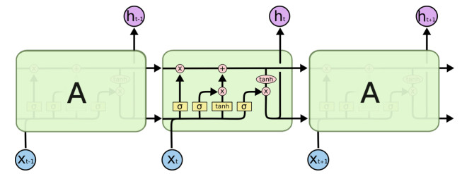
    [21] C. Olah, Understanding LSTM Networks, 2015. Available from: http://colah.github.io/posts/2015-08-Understanding-LSTMs.
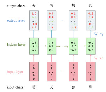
    [22] A. Karpathy,The unreasonable effectiveness of recurrent neural networks, 2015. Available from: http://karpathy.github.io/2015/05/21/rnn-effectiveness.
    [23] Q. Y. Du, The application of the thirteen rhymes in singing technique, Journal of Xingyi Normal University for Nationalities, (2010), in Chinese.
  • This article has been cited by:

    1. Shuyun Jiao, Mingzhan Huang, An SIHR epidemic model of the COVID-19 with general population-size dependent contact rate, 2020, 5, 2473-6988, 6714, 10.3934/math.2020431
    2. Chaofan Qian, Yuhui Hu, Novel stability criteria on nonlinear density-dependent mortality Nicholson’s blowflies systems in asymptotically almost periodic environments, 2020, 2020, 1029-242X, 10.1186/s13660-019-2275-4
    3. Qian Cao, Xiaojin Guo, Anti-periodic dynamics on high-order inertial Hopfield neural networks involving time-varying delays, 2020, 5, 2473-6988, 5402, 10.3934/math.2020347
    4. Manickam Iswarya, Ramachandran Raja, Grienggrai Rajchakit, Jinde Cao, Jehad Alzabut, Chuangxia Huang, Existence, Uniqueness and Exponential Stability of Periodic Solution for Discrete-Time Delayed BAM Neural Networks Based on Coincidence Degree Theory and Graph Theoretic Method, 2019, 7, 2227-7390, 1055, 10.3390/math7111055
    5. Yadan Zhang, Minghui Jiang, Xue Fang, A New Fixed-Time Stability Criterion and Its Application to Synchronization Control of Memristor-Based Fuzzy Inertial Neural Networks with Proportional Delay, 2020, 52, 1370-4621, 1291, 10.1007/s11063-020-10305-9
    6. Qian Cao, Guoqiu Wang, Chaofan Qian, New results on global exponential stability for a periodic Nicholson’s blowflies model involving time-varying delays, 2020, 2020, 1687-1847, 10.1186/s13662-020-2495-4
    7. Hong Zhang, Qian Cao, Hedi Yang, Asymptotically almost periodic dynamics on delayed Nicholson-type system involving patch structure, 2020, 2020, 1029-242X, 10.1186/s13660-020-02366-0
    8. Anbalagan Pratap, Ramachandran Raja, Jehad Alzabut, Jinde Cao, Grienggrai Rajchakit, Chuangxia Huang, Mittag‐Leffler stability and adaptive impulsive synchronization of fractional order neural networks in quaternion field, 2020, 43, 0170-4214, 6223, 10.1002/mma.6367
    9. Chaofan Qian, New periodic stability for a class of Nicholson's blowflies models with multiple different delays, 2020, 0020-7179, 1, 10.1080/00207179.2020.1766118
    10. Umesh Kumar, Subir Das, Chuangxia Huang, Jinde Cao, Fixed-time synchronization of quaternion-valued neural networks with time-varying delay, 2020, 476, 1364-5021, 20200324, 10.1098/rspa.2020.0324
    11. Chuangxia Huang, Luanshan Yang, Jinde Cao, Asymptotic behavior for a class of population dynamics, 2020, 5, 2473-6988, 3378, 10.3934/math.2020218
    12. M. Syed Ali, G. Narayanan, Sumit Saroha, Bandana Priya, Ganesh Kumar Thakur, Finite-time stability analysis of fractional-order memristive fuzzy cellular neural networks with time delay and leakage term, 2021, 185, 03784754, 468, 10.1016/j.matcom.2020.12.035
    13. Sudesh Kumari, Renu Chugh, Jinde Cao, Chuangxia Huang, Multi Fractals of Generalized Multivalued Iterated Function Systems in b-Metric Spaces with Applications, 2019, 7, 2227-7390, 967, 10.3390/math7100967
    14. M. Iswarya, R. Raja, G. Rajchakit, J. Cao, J. Alzabut, C. Huang, A perspective on graph theory-based stability analysis of impulsive stochastic recurrent neural networks with time-varying delays, 2019, 2019, 1687-1847, 10.1186/s13662-019-2443-3
    15. Xin Long, Novel stability criteria on a patch structure Nicholson’s blowflies model with multiple pairs of time-varying delays, 2020, 5, 2473-6988, 7387, 10.3934/math.2020473
    16. Lihong Huang, Huili Ma, Jiafu Wang, Chuangxia Huang, GLOBAL DYNAMICS OF A FILIPPOV PLANT DISEASE MODEL WITH AN ECONOMIC THRESHOLD OF INFECTED-SUSCEPTIBLE RATIO, 2020, 10, 2156-907X, 2263, 10.11948/20190409
    17. Xin Yang, Shigang Wen, Xian Zhao, Chuangxia Huang, Systemic importance of financial institutions: A complex network perspective, 2020, 545, 03784371, 123448, 10.1016/j.physa.2019.123448
    18. Wentao Wang, Wei Chen, Persistence and extinction of Markov switched stochastic Nicholson’s blowflies delayed differential equation, 2020, 13, 1793-5245, 2050015, 10.1142/S1793524520500151
    19. Xin Yang, Shigang Wen, Zhifeng Liu, Cai Li, Chuangxia Huang, Dynamic Properties of Foreign Exchange Complex Network, 2019, 7, 2227-7390, 832, 10.3390/math7090832
    20. Qian Cao, Guoqiu Wang, Dynamic analysis on a delayed nonlinear density-dependent mortality Nicholson's blowflies model, 2020, 0020-7179, 1, 10.1080/00207179.2020.1725134
    21. Hong Zhang, Chaofan Qian, Convergence analysis on inertial proportional delayed neural networks, 2020, 2020, 1687-1847, 10.1186/s13662-020-02737-3
    22. Ajendra singh, Jitendra Nath Rai, Stability of Fractional Order Fuzzy Cellular Neural Networks with Distributed Delays via Hybrid Feedback Controllers, 2021, 1370-4621, 10.1007/s11063-021-10460-7
    23. Qian Cao, Xin Long, New convergence on inertial neural networks with time-varying delays and continuously distributed delays, 2020, 5, 2473-6988, 5955, 10.3934/math.2020381
    24. Chuangxia Huang, Xiaoguang Yang, Jinde Cao, Stability analysis of Nicholson’s blowflies equation with two different delays, 2020, 171, 03784754, 201, 10.1016/j.matcom.2019.09.023
    25. Jian Zhang, Chuangxia Huang, Dynamics analysis on a class of delayed neural networks involving inertial terms, 2020, 2020, 1687-1847, 10.1186/s13662-020-02566-4
    26. Qian Wang, Hui Wei, Zhiwen Long, A non-reduced order approach to stability analysis of delayed inertial genetic regulatory networks, 2021, 33, 0952-813X, 227, 10.1080/0952813X.2020.1735531
    27. Jiafu Wang, Su He, Lihong Huang, Limit Cycles Induced by Threshold Nonlinearity in Planar Piecewise Linear Systems of Node-Focus or Node-Center Type, 2020, 30, 0218-1274, 2050160, 10.1142/S0218127420501606
    28. Gang Yang, Qian Cao, Stability for patch structure Nicholson’s blowflies systems involving distinctive maturation and feedback delays, 2020, 0952-813X, 1, 10.1080/0952813X.2020.1836032
    29. Chuangxia Huang, Xin Long, Jinde Cao, Stability of antiperiodic recurrent neural networks with multiproportional delays, 2020, 43, 0170-4214, 6093, 10.1002/mma.6350
    30. Qian Cao, Guoqiu Wang, New findings on global exponential stability of inertial neural networks with both time-varying and distributed delays, 2021, 0952-813X, 1, 10.1080/0952813X.2021.1883744
    31. Ruihan Chen, Song Zhu, Yongqiang Qi, Yuxin Hou, Reachable set bounding for neural networks with mixed delays: Reciprocally convex approach, 2020, 125, 08936080, 165, 10.1016/j.neunet.2020.02.005
    32. Shigang Wen, Yu Tan, Mengge Li, Yunke Deng, Chuangxia Huang, Analysis of Global Remittance Based on Complex Networks, 2020, 8, 2296-424X, 10.3389/fphy.2020.00085
    33. Zhenhua Duan, Changjin Xu, Anti-periodic behavior for quaternion-valued delayed cellular neural networks, 2021, 2021, 1687-1847, 10.1186/s13662-021-03327-7
    34. Yi Wang, Jinde Cao, Gang Huang, Further dynamic analysis for a network sexually transmitted disease model with birth and death, 2019, 363, 00963003, 124635, 10.1016/j.amc.2019.124635
    35. Luogen Yao, Qian Cao, Anti-periodicity on high-order inertial Hopfield neural networks involving mixed delays, 2020, 2020, 1029-242X, 10.1186/s13660-020-02444-3
    36. Anbalagan Pratap, Ramachandran Raja, Jinde Cao, Chuangxia Huang, Michal Niezabitowski, Ovidiu Bagdasar, Stability of discrete‐time fractional‐order time‐delayed neural networks in complex field, 2021, 44, 0170-4214, 419, 10.1002/mma.6745
    37. Luogen Yao, Global exponential stability on anti-periodic solutions in proportional delayed HIHNNs, 2021, 33, 0952-813X, 47, 10.1080/0952813X.2020.1721571
    38. Yanli Xu, Qian Cao, Xiaojin Guo, Stability on a patch structure Nicholson’s blowflies system involving distinctive delays, 2020, 105, 08939659, 106340, 10.1016/j.aml.2020.106340
    39. Yanli Xu, Qian Cao, Global asymptotic stability for a nonlinear density-dependent mortality Nicholson’s blowflies system involving multiple pairs of time-varying delays, 2020, 2020, 1687-1847, 10.1186/s13662-020-02569-1
    40. Sudesh Kumari, Renu Chugh, Jinde Cao, Chuangxia Huang, On the construction, properties and Hausdorff dimension of random Cantor one pth set, 2020, 5, 2473-6988, 3138, 10.3934/math.2020202
    41. A. Pratap, R. Raja, Jinde Cao, J. Alzabut, Chuangxia Huang, Finite-time synchronization criterion of graph theory perspective fractional-order coupled discontinuous neural networks, 2020, 2020, 1687-1847, 10.1186/s13662-020-02551-x
    42. Qian Cao, Guoqiu Wang, Hong Zhang, Shuhua Gong, New results on global asymptotic stability for a nonlinear density-dependent mortality Nicholson’s blowflies model with multiple pairs of time-varying delays, 2020, 2020, 1029-242X, 10.1186/s13660-019-2277-2
    43. Rundong Zhao, Qiming Liu, Meici Sun, Dynamical behavior of a stochastic SIQS epidemic model on scale-free networks, 2021, 1598-5865, 10.1007/s12190-021-01550-9
    44. Xianhui Zhang, Convergence analysis of a patch structure Nicholson’s blowflies system involving an oscillating death rate, 2021, 0952-813X, 1, 10.1080/0952813X.2021.1908433
    45. Roberto Galizia, Petri T. Piiroinen, Regions of Reduced Dynamics in Dynamic Networks, 2021, 31, 0218-1274, 2150080, 10.1142/S0218127421500802
    46. Jian Zhang, Ancheng Chang, Gang Yang, Periodicity on Neutral-Type Inertial Neural Networks Incorporating Multiple Delays, 2021, 13, 2073-8994, 2231, 10.3390/sym13112231
    47. Jiaying Zhou, Yi Zhao, Yong Ye, Yixin Bao, Bifurcation Analysis of a Fractional-Order Simplicial SIRS System Induced by Double Delays, 2022, 32, 0218-1274, 10.1142/S0218127422500687
    48. Shuping Li, Xiaorong Zhao, Ruixia Zhang, Site-bond percolation model of epidemic spreading with vaccination in complex networks, 2022, 85, 0303-6812, 10.1007/s00285-022-01816-1
    49. Lian Duan, Lihong Huang, Chuangxia Huang, Spatial dynamics of a diffusive SIRI model with distinct dispersal rates and heterogeneous environment, 2021, 20, 1534-0392, 3539, 10.3934/cpaa.2021120
    50. Jie Li, Jiu Zhong, Yong-Mao Ji, Fang Yang, A new SEIAR model on small-world networks to assess the intervention measures in the COVID-19 pandemics, 2021, 25, 22113797, 104283, 10.1016/j.rinp.2021.104283
    51. Chaouki Aouiti, Mahjouba Ben Rezeg, Impulsive multidirectional associative memory neural networks: New results, 2021, 14, 1793-5245, 10.1142/S1793524521500601
    52. Hong Zhang, Qian Cao, Hedi Yang, Dynamics analysis of delayed Nicholson-type systems involving patch structure and asymptotically almost periodic environments, 2022, 34, 0952-813X, 725, 10.1080/0952813X.2021.1924869
    53. Reinhard Schlickeiser, Martin Kröger, Determination of a Key Pandemic Parameter of the SIR-Epidemic Model from Past COVID-19 Mutant Waves and Its Variation for the Validity of the Gaussian Evolution, 2023, 5, 2624-8174, 205, 10.3390/physics5010016
    54. Xiaojin Guo, Chuangxia Huang, Jinde Cao, Nonnegative periodicity on high-order proportional delayed cellular neural networks involving D operator, 2020, 6, 2473-6988, 2228, 10.3934/math.2021135
    55. Qian Cao, Attractivity analysis on a neoclassical growth system incorporating patch structure and multiple pairs of time-varying delays, 2021, 14173875, 1, 10.14232/ejqtde.2021.1.76
    56. Reinhard Schlickeiser, Martin Kröger, Key Epidemic Parameters of the SIRV Model Determined from Past COVID-19 Mutant Waves, 2023, 3, 2673-8112, 592, 10.3390/covid3040042
    57. Shixiang Han, Guanghui Yan, Huayan Pei, Wenwen Chang, Dynamical Analysis of an Improved Bidirectional Immunization SIR Model in Complex Network, 2024, 26, 1099-4300, 227, 10.3390/e26030227
    58. Guangyu Li, Haifeng Du, Jiarui Fan, Xiaochen He, Wenhua Wang, The Effect of Fangcang Shelter Hospitals under Resource Constraints on the Spread of Epidemics, 2023, 20, 1660-4601, 5802, 10.3390/ijerph20105802
    59. Chuangxia Huang, Jiafu Wang, Lihong Huang, Asymptotically almost periodicity of delayed Nicholson-type system involving patch structure, 2020, 2020, 1072-6691, 61, 10.58997/ejde.2020.61
    60. 德玉 郭, Construction and Dynamic Analysis of a Class of Hepatitis C Model with Population Heterogeneity, 2023, 12, 2324-7991, 4665, 10.12677/AAM.2023.1211458
    61. Guojin Wang, Wei Yao, An application of small-world network on predicting the behavior of infectious disease on campus, 2024, 9, 24680427, 177, 10.1016/j.idm.2023.12.007
    62. Bingjie Wu, Liang’an Huo, Studying the impact of individual emotional states on the co-evolution of information, behavior and disease in multiplex networks, 2025, 03784371, 130480, 10.1016/j.physa.2025.130480
    63. Samuel Lopez, Natalia L. Komarova, An optimal network that promotes the spread of an advantageous variant in an SIR epidemic, 2025, 00225193, 112095, 10.1016/j.jtbi.2025.112095
  • Reader Comments
  • © 2019 the Author(s), licensee AIMS Press. This is an open access article distributed under the terms of the Creative Commons Attribution License (http://creativecommons.org/licenses/by/4.0)
通讯作者: 陈斌, bchen63@163.com
  • 1. 

    沈阳化工大学材料科学与工程学院 沈阳 110142

  1. 本站搜索
  2. 百度学术搜索
  3. 万方数据库搜索
  4. CNKI搜索

Metrics

Article views(8606) PDF downloads(860) Cited by(15)

Figures and Tables

Figures(8)  /  Tables(3)

Other Articles By Authors

/

DownLoad:  Full-Size Img  PowerPoint
Return
Return

Catalog