We present a general computational framework that enables one to generate realistic 3D microstructure models of heterogeneous materials from limited morphological information via stochastic optimization. In our framework, the 3D material microstructure is represented as a 3D array, whose entries indicate the local state of that voxel. The limited structural data obtained in various experiments correspond to different mathematical transformations of the 3D array. Reconstructing the 3D material structure from such limited data is formulated as an inverse problem, originally proposed by Yeong and Torquato [Phys. Rev. E 57, 495 (1998)], which is solved using the simulated annealing procedure. The utility, versatility and robustness of our general framework are illustrated by reconstructing a polycrystalline microstructure from 2D EBSD micrographs and a binary metallic alloy from limited angle projections. Our framework can be also applied in the reconstructions based on small-angle x-ray scattering (SAXS) data and has ramifications in 4D materials science (e.g., charactering structural evolution over time).
Citation: Jiao Yang. Three-Dimensional Heterogeneous Material Microstructure Reconstruction from Limited Morphological Information via Stochastic Optimization[J]. AIMS Materials Science, 2014, 1(1): 28-40. doi: 10.3934/matersci.2014.1.28
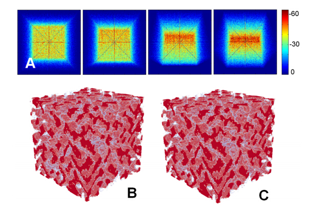
We present a general computational framework that enables one to generate realistic 3D microstructure models of heterogeneous materials from limited morphological information via stochastic optimization. In our framework, the 3D material microstructure is represented as a 3D array, whose entries indicate the local state of that voxel. The limited structural data obtained in various experiments correspond to different mathematical transformations of the 3D array. Reconstructing the 3D material structure from such limited data is formulated as an inverse problem, originally proposed by Yeong and Torquato [Phys. Rev. E 57, 495 (1998)], which is solved using the simulated annealing procedure. The utility, versatility and robustness of our general framework are illustrated by reconstructing a polycrystalline microstructure from 2D EBSD micrographs and a binary metallic alloy from limited angle projections. Our framework can be also applied in the reconstructions based on small-angle x-ray scattering (SAXS) data and has ramifications in 4D materials science (e.g., charactering structural evolution over time).

| [1] | Christensen RM (1979) Mechanics of Composite Materials.New York: Wiley . |
| [2] | Nemat-Nasser S, Hori M (1999) Micromechanics: Overall Properties of Heterogeneous Solids.Elsevier Science . |
| [3] | Torquato S (2002) Random Heterogeneous Materials: Microstructure and Macroscopic Properties.New York: Springer . |
| [4] | Sahimi M (2003) Heterogeneous Materials I: Linear Transport and Optical Properties, and II: Nonlinear and Breakdown Properties and Atomistic Modeling.New York: Springer . |
| [5] | Millar DIA (2012) Energetic Materials at Extreme Conditions.Springer Ph.D. Thesis . |
| [6] | Haymes RC (1971) Introduction to Space Science.New York: John Wiley and Sons Inc . |
| [7] | Thornton K, Poulsen HF (2008) Three-dimensional materials science: An intersection of three-dimensional reconstructions and simulations.MRS Bull 33: 587. |
| [8] | Brandon D, Kaplan WD (1999) Microstructural Characterization of Materials.New York: John Wiley and Sons . |
| [9] | Baruchel J, Bleuet P, Bravin A, et al. (2008) Advances in synchrotron hard x-ray based imaging.C R Physique 9: 624. |
| [10] | Kinney JH, Nichols MC (1992) X-ray tomographic microscopy (XTM) using synchrotron radiation.Annu Rev Mater Sci 22: 121. |
| [11] | Kak A, Slaney M (1988) Principles of Computerized Tomographic Imaging.IEEE Press . |
| [12] | Babout L, Maire E, Buffière JY (2001) Characterisationby X-ray computed tomography of decohesion, porosity growth and coalescence in model metal matrix composites.Acta Mater 49: 2055. |
| [13] | Borbély A, Csikor FF, Zabler S, et al. (2004) Three-dimensional characterization of the microstructure of a metal-matrix composite by holotomography.Mater Sci Engng A 367: 40. |
| [14] | Kenesei P, Biermann H, Borbély A (2005) Structure-property relationship in particle reinforced metal-matrix composites based on holotomography.Scr Mater 53: 787. |
| [15] | Weck A, Wilkinson DS, Maire E (2008) Visualization by x-ray tomography of void growth and coalescence leading to fracture in model materials.Acta Mater 56: 2919. |
| [16] | Toda H, Yamamoto S, Kobayashi M (2008) Direct measurement procedure for three-dimensional local crack driving force using synchrotron X-ray microtomography.Acta Mater 56: 6027. |
| [17] | Williams JJ, Flom Z, Amell AA (2010) Damage evolution in SiC particle reinforced Al alloy matrix composites by X-ray synchrotron tomography.Acta Mater 58: 6194. |
| [18] | Williams JJ, Yazzie KE, Phillips NC (2011) On the correlation between fatigue striation spacing and crack crowth rate: A three-dimensional (3-D) X-ray synchrotron tomography study.Metal Mater Trans 42: 3845. |
| [19] | Williams JJ, Yazzie KE, Phillips NC, et al.Understanding fatigue crack growth in aluminum alloys by in situ x-ray synchrotron tomography.Int J Fatigue in press . |
| [20] | Groeber M, Ghosh S, Uchic MD (2008) A framework for automated analysis and simulation of 3D polycrystalline microstructures. I: Statistical characterization.Acta Mater 56: 1257. |
| [21] | Groeber M, Ghosh S, Uchic MD (2008) A framework for automated analysis and simulation of 3D polycrystalline microstructures. II: Synthetic structure generation.Acta Mater 56: 1274. |
| [22] | Niezgoda SR, Fullwood DT, Kalidindi SR (2008) Delineation of the space of 2-point correlations in a composite material system.Acta Mater 56: 5286-5292. |
| [23] | Debye P, Anderson HR, Brumberger H (1957) Scattering by an inhomogeneous solid. II. The correlation function and its applications.J. Appl Phys 28: 679-683. |
| [24] | Yeong CLY, Torquato S (1998) Reconstructing random media.Phys Rev E 57: 495. |
| [25] | Yeong CLY, Torquato S (1998) Reconstructing random media: II. Three-dimensional reconstruction from two-dimensional cuts.Phys Rev E 58: 224. |
| [26] | Jiao Y, Stillinger FH, Torquato S (2007) Modeling heterogeneous materials via two-point correlation functions: Basic principles.Phys Rev E 76: 031110. |
| [27] | Jiao Y, Stillinger FH, Torquato S (2008) Modeling heterogeneous materials via two-point correlation functions: II. Algorithmic details and applications.Phys Rev E 77: 031135. |
| [28] | Jiao Y, Stillinger FH, Torquato S (2008) A superior descriptor of random textures and its predictive capacity.Proc Natl Acad Sci USA 106: 17634. |
| [29] | Roberts AP (1997) Statistical reconstruction of three-dimensional porous media from twodimensional images.Phys Rev E 56: 3203-3212. |
| [30] | Fullwood DT, Niezgoda SR, Kalidindi SR (2008) Microstructure reconstructions from 2-point statistics using phase-recovery algorithms.Acta Mater 56: 942-948. |
| [31] | Alireza H, Aliakbar S, Farhad A. (2011) Farhadpour A multiple-point statistics algorithm for 3D pore space reconstruction from 2D images.Advances in Water Resources 34: 1256-1267. |
| [32] | Tahmasebi P, Sahimi M (2013) Cross-correlation function for accurate reconstruction of heterogeneous media.Phys Rev Lett 110: 078002. |
| [33] | Torquato S (1986) Interfacial surface statistics arising in diffusion and flow problems in porous media.J Chem Phys 85: 4622. |
| [34] | Lu B, Torquato S (1992) Lineal path function for random heterogeneous materials.Phys Rev A 45: 922. |
| [35] | Torquato S, Avellaneda M (1991) Diffusion and reaction in heterogeneous media: Pore-size distribution, relaxation rimes, and mean survival time.J Chem Phys 95: 6477. |
| [36] | Prager S (1963) Interphase transfer in stationary two-phase media.Chem Eng Sci 18: 228. |
| [37] | Torquato S, Beasley JD, Chiew YC (1988) Two-point cluster function for continuum percolation.J Chem Phys 88: 6540. |
| [38] | Singh SS, Williams JJ, Jiao Y, et al. (2012) Modeling anisotropic multiphase heterogeneous materials via directional correlation functions: Simulations and experimental verification.Metall Mater Trans 43 A: 4470-4474. |
| [39] | Jiao Y, Pallia E, Chawla N (2013) Modeling and predicting microstructure evolution in lead/tin alloy via correlation functions and stochastic material reconstruction.Acta Mater 61: 3370. |
| [40] | Liu Y, Greene MS, Chen W, et al. (2013) Computational microstructure characterization and reconstruction for stochastic multiscale material design.Computer-Aided Design 45: 65. |
| [41] | Mikdam A, Belouettar R, Fiorelli D, et al. (2013) A tool for design of heterogeneous materials with desired physical properties using statistical continuum theory.Mater Sci Eng A 564: 493. |
| [42] | Kirkpatrick S, Gelatt CD, Vecchi MP (1983) Optimization by simulated annealing.Science 220: 671-680. |
| [43] | Sheehan N, Torquato S (2001) Generating Microstructures with Specified Correlation Functions.J Appl Phys 89: 53. |
| [44] | Rozman MG, Utz M (2002) Uniqueness of reconstruction of multiphase morphologies from two-point correlation functions.Physl Rev Lett 89: 135501. |
| [45] | Manko HH (2001) Solders and Soldering: Materials, Design, Production, and Analysis for Reliable Bonding.New York: McGraw-Hill . |
| [46] | Gommes CJ (2013) Three-dimensional reconstruction of liquid phases in disordered mesopores using in situ small-angle scattering.J Appl Cryst 46: 493-504. |
| [47] | Zhang H, Srolovitz DJ, Douglas JF (2009) Grain boundaries exhibit the dynamics of glass-forming liquids.Proc Natl Acad Sci USA 106: 7729-7734. |
| [48] | Chen Z, Chu KT, Srolovitz DJ (2010) Dislocation climb strengthening in systems with immobile obstacles: Three-dimensional level-set simulation study.Phys Rev B 81: 054104. |
Figures(5)

Jiao Yang. Three-Dimensional Heterogeneous Material Microstructure Reconstruction from Limited Morphological Information via Stochastic Optimization[J]. AIMS Materials Science, 2014, 1(1): 28-40. doi: 10.3934/matersci.2014.1.28


 DownLoad: