S-type | BS | B-type | |
The rapid urban development in San Juan, Puerto Rico, initiated by Operation Bootstrap in the late 1940s, has profoundly impacted the historical memory and identity of its inhabitants. This study examines the socioeconomic and cultural effects of transforming the El Fanguito and Tokio slums into the financial hub of Hato Rey. Through a combination of existing interviews and new testimonies, the research explores how the displacement of long-standing communities disrupted residents' sense of belonging and continuity. The findings reveal patterns of exploitation, cultural imperialism, and persistent neglect by the authorities. Despite the challenges, the current residents of Caño Martín Peña have maintained resilience and a collective identity, advocating for their rights and working towards a better future. This study underscores the need for urban planning that balances economic growth with heritage preservation, ensuring that development policies do not erase the cultural and social fabric of the communities.
Citation: Maria Helena Luengo-Duque. Erasing roots: The impact of urban development on historical memory and identity in San Juan[J]. Urban Resilience and Sustainability, 2025, 3(1): 26-56. doi: 10.3934/urs.2025002
[1] | Shan Jiang, Li Liang, Meiling Sun, Fang Su . Uniform high-order convergence of multiscale finite element computation on a graded recursion for singular perturbation. Electronic Research Archive, 2020, 28(2): 935-949. doi: 10.3934/era.2020049 |
[2] | Li-Bin Liu, Ying Liang, Jian Zhang, Xiaobing Bao . A robust adaptive grid method for singularly perturbed Burger-Huxley equations. Electronic Research Archive, 2020, 28(4): 1439-1457. doi: 10.3934/era.2020076 |
[3] | Jun Pan, Yuelong Tang . Two-grid H1-Galerkin mixed finite elements combined with L1 scheme for nonlinear time fractional parabolic equations. Electronic Research Archive, 2023, 31(12): 7207-7223. doi: 10.3934/era.2023365 |
[4] | Hongze Zhu, Chenguang Zhou, Nana Sun . A weak Galerkin method for nonlinear stochastic parabolic partial differential equations with additive noise. Electronic Research Archive, 2022, 30(6): 2321-2334. doi: 10.3934/era.2022118 |
[5] | Xiu Ye, Shangyou Zhang, Peng Zhu . A weak Galerkin finite element method for nonlinear conservation laws. Electronic Research Archive, 2021, 29(1): 1897-1923. doi: 10.3934/era.2020097 |
[6] | Leilei Wei, Xiaojing Wei, Bo Tang . Numerical analysis of variable-order fractional KdV-Burgers-Kuramoto equation. Electronic Research Archive, 2022, 30(4): 1263-1281. doi: 10.3934/era.2022066 |
[7] | Derrick Jones, Xu Zhang . A conforming-nonconforming mixed immersed finite element method for unsteady Stokes equations with moving interfaces. Electronic Research Archive, 2021, 29(5): 3171-3191. doi: 10.3934/era.2021032 |
[8] | Chunmei Wang . Simplified weak Galerkin finite element methods for biharmonic equations on non-convex polytopal meshes. Electronic Research Archive, 2025, 33(3): 1523-1540. doi: 10.3934/era.2025072 |
[9] | Yue Feng, Yujie Liu, Ruishu Wang, Shangyou Zhang . A conforming discontinuous Galerkin finite element method on rectangular partitions. Electronic Research Archive, 2021, 29(3): 2375-2389. doi: 10.3934/era.2020120 |
[10] | Yan Yang, Xiu Ye, Shangyou Zhang . A pressure-robust stabilizer-free WG finite element method for the Stokes equations on simplicial grids. Electronic Research Archive, 2024, 32(5): 3413-3432. doi: 10.3934/era.2024158 |
The rapid urban development in San Juan, Puerto Rico, initiated by Operation Bootstrap in the late 1940s, has profoundly impacted the historical memory and identity of its inhabitants. This study examines the socioeconomic and cultural effects of transforming the El Fanguito and Tokio slums into the financial hub of Hato Rey. Through a combination of existing interviews and new testimonies, the research explores how the displacement of long-standing communities disrupted residents' sense of belonging and continuity. The findings reveal patterns of exploitation, cultural imperialism, and persistent neglect by the authorities. Despite the challenges, the current residents of Caño Martín Peña have maintained resilience and a collective identity, advocating for their rights and working towards a better future. This study underscores the need for urban planning that balances economic growth with heritage preservation, ensuring that development policies do not erase the cultural and social fabric of the communities.
We will present a weak Galerkin finite element method for the following parabolic singularly perturbed convection-reaction-diffusion problem:
{∂tu−εΔu+b⋅∇u+cu=f(x,y,t)inΩ×(0,T],u=0on∂Ω×(0,T],u(x,0)=u0in¯Ω, | (1.1) |
where Ω=(0,1)2, 0<ε≪1, and T>0 is a constant. Assume b=b(x,y),c=c(x,y), and u0=u0(x,y) are sufficiently smooth functions on Ω, and
b=(b1(x,y),b2(x,y))≥(β1,β2),c−12∇⋅b≥c0>0on Ω, | (1.2) |
for some constants β1,β2, and c0. The parabolic convection-dominated problem (1.1) has been utilized in a broad range of applied mathematics and engineering including fluid dynamics, electrical engineering, and the transport problem [1,2].
In general, the solution of the problem (1.1) will have abrupt changes along the boundary. In other words, the solution exhibits boundary/interior layers near the boundary of Ω. We are only interested in the boundary layers by excluding the interior layers which can be accomplished by assuming some extra compatible conditions on the data; see, e.g., [1,3]. The standard numerical schemes including the finite element method give unsatisfactory numerical results due to the boundary layers. Some nonphysical oscillations in the numerical solution can occur even on adapted meshes, and it is not easy to solve efficiently the resulting discrete system [4]. There are many numerical schemes for solving convection-dominated problems efficiently and accurately in the literature. These methods include Galerkin finite element methods [5,6,7], weak Galerkin finite element methods (WG-FEMs) [8,9,10], the streamline upwind Petrov-Galerkin (SUPG) [11,12], and the discontinuous Galerkin (DG) methods [13,14,15]. Among these numerical methods, the standard WG-FEM introduced in [16] is also an effective and flexible numerical algorithm for solving PDEs. Recently, the WG methods demonstrate robust and stable discretizations for singularly perturbed problems. In fact, while the WG-FEM and the hybridizable discontinuous Galerkin share something in common, the WG-FEM seems more appropriate for solving the time dependent singularly perturbed problems since the inclusion of the convective term in the context of hybridized methods is not straightforward and makes the analysis more subtle. Errors estimates of arbitrary-order methods, including the virtual element method (VEM), are typically limited by the regularity of the exact solution. A distinctive feature of the WG-FEM lies in its use of weak function spaces. Moreover, hybrid high-order (HHO) methods have similar features with WG-FEMs. In fact, the reconstruction operator in the HHO method and the weak gradient operator in WG methods are closely related, and that the main difference between HHO and WG methods lies in the choice of the discrete unknowns and the design of the stabilization operator [17]. Notably, in weak Galerkin methods, weak derivatives are used instead of strong derivatives in variational form for underlying PDEs and adding parameter free stabilization terms. Considering the application of the WG method, various PDEs arising from the mathematical modeling of practical problems in science are solved numerically via WG-FEMs using the concept of weak derivatives. There exist many papers on such PDEs including elliptic equations in [16,18,19], parabolic equations [20,21,22], hyperbolic equations [23,24], etc.
However, to the best of the author's knowledge, there is no work regarding the uniform convergence results of the fully-discrete WG-FEM for singularly perturbed parabolic problems on layer-adapted meshes. This paper uses three layer-adapted meshes defined through mesh generating functions, namely, Shishkin-type meshes, Bakhvalov-Shishkin type meshes and Bakhvalov-type meshes given in [25]. The error estimates in this work show that one has optimal order of convergence for Bakhvalov-Shishkin type meshes and Bakhvalov-type meshes while almost optimal convergence for Shishkin-type meshes. The main ingredient of the error analysis is the use of the vertices-edges interpolation of Lin [26]. The main advantage of this interpolation operator is that we have sharper error bounds compared with the classical interpolation operators. For the sake of simplicity, the Crank–Nicolson method is used for time discretization. This scheme yields optimal order estimates for fully-discrete WG-FEM. As an alternative, one can apply a discontinuous Galerkin method in time and present optimal order estimates for the fully-discrete scheme [27].
The rest of the paper is organized as follows. In Section 2, we introduce some notations and recall some definitions. The regularity of the solution is also summarized and three layer-adapted meshes have been introduced in Section 2. Also, we define the weak gradient and weak convection operators, and using these concepts we define our bilinear forms. In Section 3, the semi-discrete WG-FEM and its stability results have been presented. Section 4 introduces a special interpolation operator and analyses interpolation error estimates. Section 5 presents error analysis of the semi-discrete WG-FEM for the problem (1.1) on the layer-adapted meshes. In Section 6, we apply the Crank-Nicolson scheme on uniform time mesh in time to obtain the fully-discrete WG-FEM, and prove uniform error estimates on the layer-adapted meshes. In Section 7, we conduct some numerical examples to validate the robustness of the WG-FEM for the problem (1.1). Summary on the contributions of this work are presented in Section 8.
Let S be a measurable subset of Ω. We shall use the classical Sobolev spaces Wr,q(S),Hr(S)=Wr,2(S),Hr0(S),Lq(S)=W0,q(S) for negative integers r>0 and 1≤q≤∞, and (⋅,⋅)S for the L2 inner product on S. The semi-norm and norm on Hr(S) are denoted by |⋅|r,S and ‖⋅‖r,S, respectively. If S=Ω, we do not write S in the subscript. Throughout the study, we shall use C as a positive generic constant, which is independent of the mesh parameters h and ε.
This section deals with the introduction of a decomposition of the solution which provides a priori information on the exact solution and its derivatives. Based on this solution decomposition, we construct layer-adapted meshes. As we noted in the introduction, the solution of (1.1) exhibits typically two exponential boundary layers at x=1 and y=1. The following lemma gives some information on the solution decomposition and bounds on the solution of (1.1) and its derivatives.
Lemma 2.1. Let k be positive integer and l∈(0,1). Assume that the solution u of the problem (1.1) belongs to the space Ck+l(QT) where QT:=Ω×(0,T]. Assume further that the solution u can be decomposed into a smooth part uR and layer components uL0,uL1, and uL1 with
u=uR+uL,uL=uL0+uL1+uL2,∀(x,y)∈¯Ω, | (2.1) |
where the smooth and layer parts satisfy
|∂i+j+ruR∂ix∂jy∂tr(x,y)|≤C | (2.2) |
|∂i+j+ruL0∂ix∂jy∂tr(x,y)|≤Cε−ie−β1(1−x)/ε, | (2.3) |
|∂i+j+ruL1∂ix∂jy∂tr(x,y)|≤Cε−je−β2(1−y)/ε, | (2.4) |
|∂i+j+ruL2∂ix∂jy∂tr(x,y)|≤Cε−(i+j)e−β1(1−x)/εe−β2(1−y)/ε, | (2.5) |
for any (x,y)∈¯Ω,t∈[0,T], and positive integers i,j,r with i+j+2r≤k, and C only depends on b,c, and f and is independent of ε. Here, uR is the regular part of u, uL0 is an exponential boundary layer along the side x=1 of Ω, uL1 is an exponential boundary layer along the side y=1, while uL2 is an exponential corner layer at (1,1).
Proof. Under some smoothness conditions and strong imposed compatibility requirements, Shishkin proved this solution decomposition; see, [1].
Let Nx and Ny be positive integers. For the sake of simplicity, we assume that Nx=Ny=N is an even integer number. We shall construct the tensor product mesh TN={Tij}i,j=1,2…,N in ¯Ω consisting of elements Tij=Ii×Kj with the intervals Ii=(xi−1,xi) and Kj=(yj−1,yj), where the mesh points are defined by
0=x0<x1<…,xNx=1,0=y0<y1<…,yNy=1. |
Since the construction of the meshes in both directions is similar, the mesh construction in x-variable is given here.
We define the transition parameter as
τ=min(12,σεβ1φ(1/2)), |
where σ⩾ is a positive constant. Here, is the degree of the polynomials used in the approximation space. The function obeys the conditions
(2.6) |
Assumption 1. Throughout this article, we assume that such that , since otherwise the analysis can be carried out using uniform mesh.
Let the mesh points be equally distributed in with intervals and distributed with intervals using the mesh generating function defined by
(2.7) |
For example, as in [25], the Shishkin-type (S-type) meshes can be deduced by while Bakhvalov-type meshes (B-type) can be recovered by taking .
We will use the mesh characterizing function defined by , which is an essential tool in our analysis below.
Following [2], we list some famous adaptive meshes including S-type, Bakhvalov-Shishkin meshes (BS-mesh), and B-type in Table 1.
S-type | BS | B-type | |
Similarly, we define the transition point in the -direction as
We first split the domain into four subdomains as in Figure 1:
Clearly, the mesh is uniform in with a mesh size of , highly anisotropic in and , while it is very fine in .
Let be the mesh sizes of the subintervals. For the sake of simplicity, we assume that . Then, one has , and we simply write for simplicity. The following technical lemmas show the smallness of the boundary layer-functions and the basic properties of the mesh sizes of the layer-adapted meshes.
Lemma 2.2. [28] Denote by for . There exists a constant independent of and such that
Lemma 2.3. [28] For the layer-adapted meshes we considered here, we have
Moreover, for
and, for the B-type mesh,
where is a constant independent of and .
A weak formulation of the problems (1.1) and (1.2) is to look for such that
(2.8) |
where the bilinear from is defined by
Based on the weak formulation (2.8), we define the WG-FEM on the layer-adapted mesh. Let be a positive integer. We define a local WG-FE space on each given by
where is the polynomials of degree on in both variables, and denotes the polynomials of degree on the edge .
Defining the WG finite element space globally on as
(2.9) |
and its subspace
The weak gradient operator can be defined on as
(2.10) |
where represents the outward unit normal , denotes the inner product on for functions and , and is the inner product on .
The weak convection operator can be defined on as
(2.11) |
For simplicity, we adapt
For and , the bilinear form is given by
(2.12) |
where and are bilinear forms defined by
with and is the penalty term given by
(2.13) |
Given a mesh rectangle , its dimensions parallel to the and -axes are written as and , respectively.
Lemma 2.4. [29] For all with , there exists a constant depending only on such that
(2.14) |
We next formulate our semi-discrete WG scheme as follows (Algorithm 1).
Algorithm 1 The semi-discrete WG-FEM for problem (1.1) |
Find such that |
where is an approximation of . |
This section is devoted to establishing the stability results of the WG-FEM defined by (2.15). Define the energy norm on the weak function space for ,
(3.1) |
Define also an equivalent norm on by
(3.2) |
The equivalence of these two norms on is given in the next lemma.
Lemma 3.1. For , one has
Proof. For , it follows from the weak gradient operator (2.10) and integration by parts that;
(3.3) |
Choosing in (3.3) and using the Cauchy-Schwartz inequality and the trace inequality (4), we arrive at
Hence, we get
Summing over all yields
From the penalty term (2.13), we get
and
As a result, for , we have
(3.4) |
Taking in (3.3) and using the Cauchy-Schwartz inequality, we get
where we have again used the trace inequality (4).
Consequently,
Summing over all yields
Therefore, we have
which implies
(3.5) |
From (3.4) and (3.5), we obtain the desired conclusion, which completes the proof.
We shall show the coercivity of the bilinear form in norm on .
Lemma 3.2. For any , the following inequality holds:
(3.6) |
Proof. For , using the weak convection derivative (2.11) and integration by parts gives
(3.7) |
and
(3.8) |
where we use the facts that , and in the last inequality.
Combining (3.7) and (3.8), and taking , we obtain
(3.9) |
From (3.9), we have
which yields (3.6) with . The proof is completed.
Therefore, the existence of a unique solution to (2.15) follows from the coercivity property of the bilinear form (3.6). As a result of the two lemmas above, the bilinear form is also coercive in the -norm in the sense that for any , there holds
(3.10) |
Lemma 3.3. If for each , then there is a constant independent of and mesh size such that the solution defined in (2.15) satisfies
(3.11) |
Proof. Choosing in (2.15) gives that
Using the Cauchy-Schwarz inequality and the coercivity (3.6) of the bilinear form ,
Integrating the above inequality with respect to the time variable , we arrive at
(3.12) |
Using the Gronwall's inequality gives the desired conclusion. We are done.
First, we define "vertices-edges' interpolation of a function on an element as follows. Let be the reference element with the vertices and the edges for . For , the approximation is given by
(4.1) |
(4.2) |
(4.3) |
The approximation operator is well-defined [30]. Thus, we can define a continuous global interpolation operator by writing
(4.4) |
where the bijective mapping is given by .
This interpolation operator has the following stability estimate [30]
(4.5) |
Since our approximation operator is continuous on , we have for . By the trace theorem, we will denote this by .
Lemma 4.1. [31] For any ,
We recall some technical results from [30].
Lemma 4.2. For any and , there exists a constant such that the vertices-edges-element approximant satisfies
for all .
Lemma 4.3. Let . The following estimates hold for any :
for all .
A careful inspection of the proof of Lemma 4.3 in [30] reveals that the following results also hold true.
Lemma 4.4. For and with , there exists a constant such that the vertices-edges-element approximant satisfies
for all .
Lemma 4.5. Let the assumption of Lemma 2.1 hold such that Then there is a constant such that the following interpolation error estimates are satisfied:
(4.6) |
(4.7) |
(4.8) |
(4.9) |
(4.10) |
(4.11) |
Proof. The proof of (4.6) follows from Lemma 4.2 and the solution decomposition (2.2) of Lemma 2.1.
Using the decay bound (2.3) of and the fact that , we have
which shows (4.7) for . Similar arguments can be applied to the layer functions and . Thus, we complete the proof of (4.7). For (4.8) and (4.9), we will prove for since the other two parts follow similarly. One can use the decay bound (2.3) of to obtain
We now shall prove (4.9). Appealing (2.3), one gets
The proof of (4.10) is a little longer. Using an inverse estimate yields
Hence, we shall estimate . With the help of the stability estimate (4.5) and the decay bound (2.3) of , we have
If , then the sum can be small as a function of but not small if . For and , we have
and when , again using the fact ,
Thus,
which proves (4.10). To prove (4.11), we use (4.7) and (4.10) to obtain
On the set , from the triangle inequality, one obtains
For , we have
For , using (4.5) and the decay property (2.3) of ,
(4.12) |
where we have used that Applying Lemma 4.2 and the decay property (2.3), we have for any
where we have used and Lemma 2.2. Similarly, one can show that (4.11) holds for as well.
For , one can prove as above . For , we obtain
Thus, we complete the proof of (4.11). The proof of the lemma is now completed.
Lemma 4.6. Let . Assume that the conditions of Lemma 4.5 hold. Then, we have
for , where denotes , or .
Proof. The first and second estimates follow from Lemma 4.3, Lemma 4.4, and the fact that . From the triangle inequality and (4.8) and (4.10) of Lemma 4.5, we have
where we have used that . This completes the proof of the third and fifth inequalities for . An inverse inequality and (4.9) and (4.10) of Lemma 4.5 lead to
where again we have used . This proves the third and fifth inequalities for . Using Lemma 4.4 with for and the decay bound (2.3) of , one can show that for any ,
Similarly, one can prove that the result holds for , too.
For , we get . For , we obtain
which completes the proof of the fourth inequality. Similarly, one can prove that the last inequality holds true. The proof is now finished.
Unlike the classical numerical methods such as FEM and the SUPG, the proposed WG-FEM does not have Galerkin orthogonality property. This results in some inconsistency errors in the error bounds. We first give a useful error equation in the following lemma.
Lemma 5.1. [31] Let solve the problem (1.1). For ,
(5.1) |
(5.2) |
(5.3) |
where
(5.4) |
(5.5) |
(5.6) |
The following error equation will be needed in the error analysis.
Lemma 5.2. Let and be the solutions of (1.1) and (2.15), respectively. For , one has
(5.7) |
where , which are defined by (5.4), (5.5), and (5.6), respectively.
Proof. Multiplying (1.1) by a test function , we arrive at
With the help of (5.1), (5.2), and (5.3), the above equation becomes
Since is continuous in , we get
Therefore, we have
(5.8) |
Subtracting (2.15) from (5.8) gives (5.7), which completes completed.
Lemma 5.3. Let be the vertex-edge-cell interpolation of the solution of the problem (1.1). Then, there holds
Proof. The solution decomposition (2.1) implies that
Using Lemma 4.2 with and Lemma 2.1,
Next, we examine the layer parts one by one. Let . From the stability property (4.5) of the interpolation operator, one has
Let . The stability property (4.5) and Lemma 4.2 with yield
Similarly, we can derive the estimates on the other layer components and . Combining the above estimates gives the desired conclusion.
Thus, we complete the proof.
We recall the following trace inequality. For any , one has
(5.9) |
Lemma 5.4. Let and be given by (2.13). Assume that the conditions of Lemma 4.5 hold. Then, one has
Proof. For the sake of simplicity, we use the following notations. Let and represent the interpolation errors of the regular and layer components of the solution. Hence, by the triangle inequality, we have
(5.10) |
With the help of the trace inequality (5.9), we have
Now, appealing the definition (2.13) of stabilization parameter and Lemma 4.6 gives
(5.11) |
where we have used that .
Using once again the trace inequality (5.9), we have
Now, appealing the definition (2.13) of stabilization parameter and Lemma 4.6 again reveals that
(5.12) |
Plugging (5.12) and (5.11) into (5.10) yields
Consequently, we have
which completes the proof.
Now, we shall prove the error bounds for the consistency errors.
Lemma 5.5. (A priori bounds) Assume that is the tensor product mesh as defined in Section 2. Then, for and we have
(5.13) |
(5.14) |
Proof. It follows from the Cauchy-Schwarz and Holder inequalities that
(5.15) |
Now, it then follows from Lemma 4.6 that
(5.16) |
Next, we consider the term . From the Cauchy-Schwarz inequality and Lemma 5.4, we have
(5.17) |
Combining (5.16) and (5.17), we get
(5.18) |
From (5.5) and (5.6) and using , we arrive at
Now, the Hölder inequality and Lemma 5.3 lead us to write
(5.19) |
The Cauchy Schwartz and inverse inequalities give
(5.20) |
Appealing the Cauchy Schwartz inequality on , we have
(5.21) |
Using the error bounds (5.20) and (5.21) in (5.19), we obtain
(5.22) |
where we have used the fact that .
Since and are continuous, we conclude that for any . Then, the Hölder inequality and Lemma 5.3 imply that
where we have used that and .
Using the Cauchy Schwartz inequality and (4.6) and (4.11) of Lemma 4.5, we obtain
The proof is completed.
By letting in (5.7), we obtain
It then follows from the estimates (5.13) and (5.14), together with Young's inequality and 3.10, that
As a result,
(5.23) |
Then, by integrating from to , we have
This result is collected in the following theorem.
Theorem 5.1. (Semi-discrete estimate) Let be the solution of (1.1)-(1.2) and be the solution of (2.15). Then, we have
In this section, we shall use the Crank-Nicolson scheme on uniform time mesh in time to derive the fully discrete approximation of the problem (1.1) and (1.2). For a given partition of the time interval for some positive integer and step length , we define
where the sequence . For simplicity, we denote by for a function We now state our fully discrete weak Galerkin finite element approximation. Find such that
(6.1) |
with and .
The following lemma shows that the Crank-Nicolson scheme is unconditionally stable in the norm.
Lemma 6.1. Let . Then, we have the following stability estimate for the fully-discrete scheme (6.1):
(6.2) |
Proof. Choosing in (6.1), and using the Cauchy-Schwarz inequality, we get
where we have used that . Using the fact that and the coercivity of the bilinear form, we have
Let be an integer. We sum the above inequality from to :
Recalling that , the result follows. The proof is now completed.
Next, we shall present the convergence analysis. To begin, we prove the error estimate of the discretization error . To this end, we need to derive an error equation involving the error .
We formulate the error equation for in the following lemma.
Lemma 6.2. For we have
(6.3) |
where ; and
Proof. From (1.1), one obtains the following equation:
(6.4) |
On each element for we test equation (6.4) against to arrive at
(6.5) |
Using a similar argument in deriving (5.8), one can show that
where we have used that since is continuous in . Thus, we get
(6.6) |
Subtracting (6.1) from (6.6) gives the conclusion. We complete the proof.
Lemma 6.3. Let . Assume that and are the solutions (1.1), (1.2), and (6.1), respectively. One has for ,
(6.7) |
Proof. Choosing in (6.3) and by the coercivity property (3.6), we find
or, equivalently,
(6.8) |
We can express the term . We write
(6.9) |
and
(6.10) |
From (6.9) and (6.10), we obtain
(6.11) |
Hence, with the aid of the Cauchy-Schwarz and the Poincare inequality, in (6.8) can be estimated as follows.
(6.12) |
where we have used the Young's inequities in the second inequality, and the estimate (6.11) and Lemma 4.5 in the second estimates of the righthand side. Applying Lemma 5.5 and Young's inequality, we obtain the estimate of the term in the righthand side of (6.8) as follows:
(6.13) |
Combining (6.8)–(6.13) yields
Let . Using the fact that , we sum the above expression from to to obtain
We complete the proof.
Theorem 6.1. Let . Assume that and are the solutions (1.1), (1.2), and (6.1), respectively. One has for ,
Proof. Choosing in (6.3) and by coercivity (3.6), we find
or, equivalently,
Thus, we have
Because , we sum up the above term from to for any fixed to get
(6.14) |
From (6.11), we have
(6.15) |
Observe that
(6.16) |
Similar to (6.13), one has
(6.17) |
It follows from Lemma 5.5, the Cauchy-Schwarz inequality, and Young's inequality that
(6.18) |
From (6.16), (6.17), and (6.18) together with , we have
(6.19) |
Combining (6.14), (6.15), and (6.19) yields that
Finally, using (6.7), we obtain
which completes the proof.
This section presents various numerical examples for the fully-discrete Crank-Nicolson WG finite element method. We used MATLAB R2020A in our the calculations. We also used the 5-point Gauss-Legendre quadrature rule for evaluating of all integrals. All the calculations were calculated using MATLAB R2016a. The systems of linear equations resulting from the discrete problems were solved by lower-upper (LU) decomposition.
We apply the fully-discrete WG-FEM on the adaptive meshes shown in Table 1. We choose and calculate the energy-norm and the -norm error , where is the error using intervals in each direction. The order of convergence (OC) is computed by the formula
The numerical errors and the order of convergences in space are also tested. In order for the space error to dominate the errors, we take for element in each direction. We list the errors in the energy norm and -norm and the order of convergence in Tables 2 and 3, respectively. These numerical results show that the order of convergence is of order and of order in the energy and norms, respectively, which support the stated error estimates in Theorem 6.1.
Shishkin | Bakhvalov- Shishkin | Bakhvalov-type | |||||
16 | – | – | – | ||||
32 | 0.90 | 0.90 | 0.93 | ||||
64 | 0.93 | 0.93 | 0.93 | ||||
128 | 0.95 | 0.95 | 0.93 | ||||
256 | 0.97 | 0.97 | 0.97 | ||||
512 | 0.99 | 1.00 | 0.99 | ||||
16 | – | – | – | ||||
32 | 1.90 | 1.80 | 1.97 | ||||
64 | 1.94 | 1.90 | 1.93 | ||||
128 | 1.96 | 1.94 | 1.93 | ||||
256 | 1.97 | 1.99 | 1.97 | ||||
512 | 2.00 | 1.99 | 2.00 | ||||
16 | – | – | – | ||||
32 | 2.90 | 2.80 | 2.90 | ||||
64 | 2.94 | 2.92 | 2.93 | ||||
128 | 2.97 | 2.97 | 2.97 | ||||
256 | 2.98 | 2.98 | 2.99 | ||||
512 | 3.00 | 3.00 | 3.00 |
Shishkin | Bakhvalov- Shishkin | Bakhvalov-type | |||||
16 | – | – | – | ||||
32 | 1.94 | 1.94 | 1.94 | ||||
64 | 1.97 | 1.97 | 1.97 | ||||
128 | 1.98 | 1.98 | 1.98 | ||||
256 | 1.99 | 1.99 | 1.99 | ||||
512 | 1.99 | 1.99 | 1.99 | ||||
16 | – | – | – | ||||
32 | 2.93 | 2.93 | 2.93 | ||||
64 | 2.97 | 2.97 | 2.97 | ||||
128 | 2.98 | 2.98 | 2.98 | ||||
256 | 2.99 | 2.99 | 2.99 | ||||
512 | 3.00 | 3.00 | 3.00 | ||||
16 | – | – | – | ||||
32 | 3.93 | 3.93 | 3.93 | ||||
64 | 3.94 | 3.94 | 3.94 | ||||
128 | 3.97 | 3.97 | 3.97 | ||||
256 | 3.99 | 3.99 | 3.99 | ||||
512 | 4.00 | 4.00 | 4.00 |
Example 7.1. Let and in the problem (1.1). We choose and such that the exact solution is
where .
In Figure 2, we plot the numerical solutions of the WG-FEM using the element on the three layer-adapted meshes given in Figure 1 for and .
We next present the temporal convergence rate for Example 7.1. In order for the temporal error to dominate the error, we take and , and use the element. We report the results in the -norm and the energy norm in Tables 4 and 5, respectively. We see that the order of convergence in time is of order , which verifies the theoretical estimate claimed in Theorem 6.1.
Shishkin | Bakhvalov- Shishkin | Bakhvalov-type | ||||
1/2 | – | – | – | |||
1/4 | 2.03 | 2.03 | 2.03 | |||
1/8 | 1.99 | 1.99 | 1.99 | |||
1/16 | 2.00 | 2.00 | 2.00 |
Shishkin | Bakhvalov- Shishkin | Bakhvalov-type | ||||
1/2 | – | – | – | |||
1/4 | 2.00 | 2.00 | 2.00 | |||
1/8 | 1.99 | 1.99 | 1.99 | |||
1/16 | 2.00 | 2.00 | 2.00 |
Lastly, we test the robustness of the WG-FEM method with respect to the small parameter for Example 7.1. We take and use the element for the values of . The results are reported in Table 6. These results show that the WG-FEM is robust with respect to the perturbation parameter .
Shishkin | Bakhvalov- Shishkin | Bakhvalov-type | |
The order of convergence via loglog plot in the energy norm and norm are plotted in Figures 3 and 4, respectively, for Example 7.2. We observe that the order of convergence of order and of order in the energy and norms, respectively, which support the stated error estimates in Theorem 6.1 as in Example 7.1. To test the temporal error, we choose and , and use the element. We present the results in the -norm and the energy norm in Tables 7 and 8, respectively. We see that the order of convergence in time is of order as claimed in Theorem 6.1.
Shishkin | Bakhvalov- Shishkin | Bakhvalov-type | ||||
1/2 | – | – | – | |||
1/4 | 1.20 | 1.20 | 1.20 | |||
1/8 | 1.70 | 1.70 | 1.70 | |||
1/16 | 2.00 | 2.00 | 2.00 |
Shishkin | Bakhvalov- Shishkin | Bakhvalov-type | ||||
1/2 | – | – | – | |||
1/4 | 1.92 | 1.92 | 1.92 | |||
1/8 | 2.01 | 2.01 | 2.01 | |||
1/16 | 2.02 | 2.02 | 2.02 |
Example 7.2. Let , , and in the problem (1.1). We take and such that the exact solution is
We also test the WG-FEM for Example 7.2 for the robustness against . The results are presented in Table 9 for and the element for the values of . Again, one sees that the WG-FEM is the parameter-uniform method.
Shishkin | Bakhvalov- Shishkin | Bakhvalov-type | |
In this paper, we present the Crack-Nicolson- WG-FEM applied to the singularly perturbed parabolic convection-dominated problems in 2D. We use the Crack-Nicolson scheme in time on uniform mesh and the WG-FEM in space on three layer-adapted meshes: Shishkin, Bakhvalov-Shishkin, and Bakhvalov meshes. We prove (almost) uniform error estimates of order in the energy norm and second order estimate in time. With the use of a special interpolation operator, the error analysis of the semi-discrete WG-FEM and the fully discrete WG-FEM have been carried out. Various numerical examples are conducted to validate the convergence rate of the proposed method.
The authors declare they have not used Artificial Intelligence (AI) tools in the creation of this article.
The authors declare there is no conflicts of interest.
[1] |
Caban PA (1989) Industrial transformation and labour relations in Puerto Rico: From 'Operation Bootstrap' to the 1970s. J Lat Am Stud 21: 559–591. https://doi.org/10.1017/S0022216X0001854X doi: 10.1017/S0022216X0001854X
![]() |
[2] | Torres EV (2023) Obligados a olvidar: Settlement and Displacement in 20th Century San Juan, Puerto Rico. Centro J 35: 7. |
[3] | Foster WZ (1948) The Crime of El Fanguito, New York: New Century Publishers. Available from: https://www.redstarpublishers.org. |
[4] |
Molano Camargo F (2016) El derecho a la ciudad: de Henri Lefebvre a los análisis sobre la ciudad capitalista contemporánea. Folios 1: 3–19. http://dx.doi.org/10.17227/01234870.44folios3.19 doi: 10.17227/01234870.44folios3.19
![]() |
[5] | Lefebvre H (1984) The Production of Space, Cambridge: Library of Congress. |
[6] |
Miller LL (2005) Root shock: How tearing up city neighborhoods hurts America and what we can do about it. J Health Polit Policy Law 30: 985–990. https://doi.org/10.1215/03616878-30-5-985 doi: 10.1215/03616878-30-5-985
![]() |
[7] | Francis D (2022) Diébédo Francis Kéré: How first Black winner of architecture's top prize is committed to building 'peaceful cities'. Available from: https://theconversation.com/diebedo-francis-kere-how-first-black-winner-of-architectures-top-prize-is-committed-to-building-peaceful-cities-179483. |
[8] | Escobar A (2011) Encountering development: The making and unmaking of the Third World, Princeton: Princeton University Press. |
[9] | Lees L, Slater T, Wyly E (2008) Gentrification, New York: Routledge. https://doi.org/10.4324/9780203940877 |
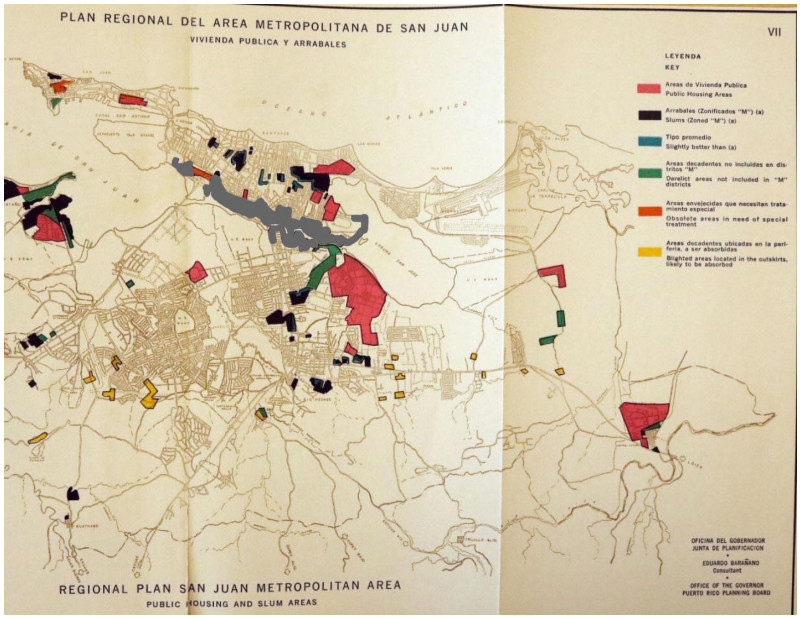
[10] | Barañano E, Board PRP (1956) Plan regional del area metropolitana de San Juan. Available from: https://issuu.com/coleccionpuertorriquena/docs/plan_regional_san_juan_-_bara_ano_1956. |
[11] | Google Earth. Available from: https://earth.google.com/web/@18.44669323,-66.04436965,11.84919169a,0d,60y,13.03335891h,94.52861367t,0r/data=CgRCAggBOgMKATBKDQj___________8BEAA. |
[12] | Archivo Virtual del Instituto de Cultura Puertorriqueña. Available from: https://www.archivoicp.com/cronicas-agpr-final. |
[13] | Cotto L (1990) La ocupación de tierras como lucha social: Los rescates de terreno en Puerto Rico: 1968–1976. Revista de Ciencias Sociales 408–428. https://api.semanticscholar.org/CorpusID:185039175 |
[14] | Scarano FA (2010) Spanish Hispaniola and Puerto Rico, In: The Oxford Handbook of Slavery in the Americas, Oxford University Press, 22–45. https://doi.org/10.1093/oxfordhb/9780199227990.013.0002 |
[15] | Sepúlveda-Rivera A, Carbonell J (1988) Cangrejos-Santurce: Historia Ilustrada de Su Desarrollo Urbano (1519–1950), Viejo San Juan P.R.: Centro de Investigaciones CARIMAR Oficina Estatal de Preservación Histórica. Available from: http://www.worldcat.org/title/cangrejos-santurce-historia-ilustrada-de-su-desarrollo-urbano-1519-1950/oclc/26398917#.W0kXfKpqg5g.mendeley. |
[16] | Acosta I (2013) Abolition of Slavery (1873), Choice Reviews Online. |
[17] |
Taylor KY (2018) How real estate segregated America. Dissent 65: 23–32. https://doi.org/10.1353/dss.2018.0071 doi: 10.1353/dss.2018.0071
![]() |
[18] | Puerto Rico Ilustrado—Digital library of the Caribbean (1936). Available from: https://dloc.com/es/AA00098206/01212/images/22. |
[19] | El Mundo 1945.02.04—El Mundo Digital Archive. Available from: https://gpa.eastview.com/crl/elmundo/?a=d&d=mndo19451103-01.1.21&e=------194-en-25--1--img-txIN-enver+azizi----1945---es--. |
[20] | El Mundo 1969.06.06—El Mundo Digital Archive. Available from: https://gpa.eastview.com/crl/elmundo/?a=d&d=mndo19690606-01.1.7&srpos=1&e=-------en-25--1--img-txIN-puerto+rico+siempre+ha+tenido+y+tiene+ahora+una+sutil+estructura+racial----1969---es--. |
[21] | El Mundo 1971.06.11—El Mundo Digital Archive. Available from: https://gpa.eastview.com/crl/elmundo/?a=d&d=mndo19710611-01.1.41&srpos=1&e=-------en-25--1--img-txIN-adem%c3%a1s+de+algunas+instituciones+religiosas+hay+otras+escuelas+privadas+que+incurren+en+el+racismo-------es--. |
[22] | 80grados+ (2020) Bomba, prohibiciones y discurso racial en los albores del siglo XX. Available from: https://www.80grados.net/bomba-prohibiciones-y-discurso-racial-en-los-albores-del-siglo-xx/. |
[23] | Brahms DP (2024) The New Old Deal: Colonial Social Welfare and Puerto Rican Poverty During the Great Depression, 1928–1941. Master's thesis, University of Maryland, College Park, 2024. |
[24] |
Duany J (2010) Anthropology in a postcolonial colony: Helen I. Safa's contribution to Puerto Rican ethnography. Caribbean Stud 38: 33–57. https://doi.org/10.1353/crb.2010.0054 doi: 10.1353/crb.2010.0054
![]() |
[25] | Jopling CF (1988) Puerto Rican Houses in Sociohistorical Perspective, Knoxville: University of Tennessee Press. |
[26] | YouTube Historia Oral del Caño Martín Peña. Available from: https://www.youtube.com/playlist?list=PLMJGEVe252Ekrwl_XJi756WoKgGyplPWF. |
[27] | Puerto Rico Historic Building Drawings Society (2024). Available from: https://www.facebook.com/PRHBDS. |
[28] | data.pr.gov, 2018. Available from: https://data.pr.gov/en/Transportaci-n/Annual-Average-Daily-Traffic-AADT-Transito-Promedi/7kaq-zyym. |
[29] | El Mundo 1949.05.07—El Mundo Digital Archive. Available from: https://gpa.eastview.com/crl/elmundo/?a=d&d=mndo19490507-01.1.1&srpos=1&e=-------en-25--1--img-txIN-%22alcaldesa+rinc%c3%b3n+tuvo+%22---------. |
[30] | Raíces del Caño (2012) En Peligro la Salud de la Gente del Caño. Available from: https://g8pr.org/wp-content/uploads/2017/05/raices-web-vol-1.pdf. |
[31] | UWM Libraries Digital Collections (1940) Puerto Rico aerial survey/Army Map Servic. Available from: https://collections.lib.uwm.edu/digital/collection/agdm/id/12469. |
[32] | EarthExplorer. Available from: https://earthexplorer.usgs.gov/. |
[33] | Wikipedia, la enciclopedia libre, Centro ceremonial indígena de Tibes. Available from: https://es.wikipedia.org/wiki/Centro_ceremonial_ind%C3%ADgena_de_Tibes. |
[34] | 80grados+ (2019) Casas jíbaras: Anotaciones sobre arquitectura y tradición. Available from: https://www.80grados.net/casas-jibaras-anotaciones-sobre-arquitectura-y-tradicion-en-puerto-rico/. |
[35] | San Juan, Puerto Rico. In the huge slum area known as "El Fangitto". Available from: https://www.loc.gov/item/2017798491/. |
[36] | Moscioni A (2005) El Fanguito, Santurce. Available from: https://upr.contentdm.oclc.org/digital/collection/Moscioni/id/1234/rec/1. |
[37] | Davis D (2016) The production of space and violence in cities of the global south: Evidence from Latin America. Nóesis: Revista de Ciencias Sociales y Humanidades 25: 1–15. |
[38] | Currie LJ (1951) Housing, Puerto Rico. Available from: https://jstor.org/stable/community.16799280. |
[39] | Dinzey-Flores ZZ (2013) Locked in, Locked out: Gated Communities in a Puerto Rican City, University of Pennsylvania Press. |
[40] | Agencia EFE (2023) La gentrificación avanza a toda velocidad en Puerto Rico. Available from: https://www.primerahora.com/noticias/gobierno-politica/notas/la-gentrificacion-avanza-a-toda-velocidad-en-puerto-rico/. |
[41] | E-Data—Departamento de Educación de PR. Available from: https://de.pr.gov/academico/secretaria-auxiliar-de-planificacion-y-rendimiento/edata/. |
[42] |
Dinzey-Flores ZZ (2011) Criminalizing communities of poor, dark women in the Caribbean: The fight against crime through Puerto Rico's public housing. Crime Prev Community Saf 13: 53–73. https://doi.org/10.1057/cpcs.2010.18 doi: 10.1057/cpcs.2010.18
![]() |
[43] |
Davis DE (2018) The routinization of violence in Latin America: Ethnographic revelations. Latin Am Res Rev 53: 211–216. https://doi.org/10.25222/larr.425 doi: 10.25222/larr.425
![]() |
[44] | Instituto de Estadísticas de PR (2024) Violent deaths reporting system Puerto Rico. Available from: https://estadisticas.pr/files/Publicaciones/Informe%20PRVDRS%202021%20English%20version.pdf. |
[45] | Data USA (2019) Puerto Rico. Available from: https://datausa.io/profile/geo/puerto-rico/. |
[46] | U.S. Department of Commerce (2018) U.S. Census Bureau QuickFacts: Puerto Rico, 2018. Available from: www.census.gov/quickfacts/PR. |
[47] |
Mattei J, Tamez M, Ríos-Bedoya CF, et al. (2018) Health conditions and lifestyle risk factors of adults living in Puerto Rico: A cross-sectional study. BMC Public Health 18: 1–12. https://doi.org/10.1186/s12889-018-5359-z doi: 10.1186/s12889-018-5359-z
![]() |
[48] | Coleman D (2008) The persistence of the past in the Albaicín: Granada's New Mosque and the question of historical relevance, In: In the Light of Medieval Spain: Islam, the West, and the Relevance of the Past, New York: Palgrave Macmillan, 157–188. https://doi.org/10.1057/9780230614086_8 |
[49] | Algoed L, Torrales MEH (2019) The land is ours. Vulnerabilization and resistance in informal settlements in Puerto Rico: Lessons from the Cano Martin Pena community land trust. Radical Hous J 1: 29–47. |
[50] |
Urban F (2015) La Perla—100 years of informal architecture in San Juan, Puerto Rico. Plan Perspect 30: 495–536. https://doi.org/10.1080/02665433.2014.1003247 doi: 10.1080/02665433.2014.1003247
![]() |
[51] | Cerreta M, La Rocca L (2021) Urban regeneration processes and social impact: A literature review to explore the role of evaluation, in Computational Science and Its Applications—ICCSA 2021, Cham: Springer, 167–182.https://doi.org/10.1007/978-3-030-86979-3_13 |
[52] |
Duany J (2000) Nation on the move: The construction of cultural identities in Puerto Rico and the diaspora. Am Ethnol 27: 5–30. https://doi.org/10.1525/ae.2000.27.1.5 doi: 10.1525/ae.2000.27.1.5
![]() |
[53] | Dovey K, van Oostrum M, Shafique T, et al. (2023) Atlas of Informal Settlement: Understanding Self-organized Urban Design, Bloomsbury Publishing. |
[54] |
Pojani D (2019) The self-built city: Theorizing urban design of informal settlements. Archnet-IJAR 13: 294–313. https://doi.org/10.1108/ARCH-11-2018-0004 doi: 10.1108/ARCH-11-2018-0004
![]() |
S-type | BS | B-type | |
Shishkin | Bakhvalov- Shishkin | Bakhvalov-type | |||||
16 | – | – | – | ||||
32 | 0.90 | 0.90 | 0.93 | ||||
64 | 0.93 | 0.93 | 0.93 | ||||
128 | 0.95 | 0.95 | 0.93 | ||||
256 | 0.97 | 0.97 | 0.97 | ||||
512 | 0.99 | 1.00 | 0.99 | ||||
16 | – | – | – | ||||
32 | 1.90 | 1.80 | 1.97 | ||||
64 | 1.94 | 1.90 | 1.93 | ||||
128 | 1.96 | 1.94 | 1.93 | ||||
256 | 1.97 | 1.99 | 1.97 | ||||
512 | 2.00 | 1.99 | 2.00 | ||||
16 | – | – | – | ||||
32 | 2.90 | 2.80 | 2.90 | ||||
64 | 2.94 | 2.92 | 2.93 | ||||
128 | 2.97 | 2.97 | 2.97 | ||||
256 | 2.98 | 2.98 | 2.99 | ||||
512 | 3.00 | 3.00 | 3.00 |
Shishkin | Bakhvalov- Shishkin | Bakhvalov-type | |||||
16 | – | – | – | ||||
32 | 1.94 | 1.94 | 1.94 | ||||
64 | 1.97 | 1.97 | 1.97 | ||||
128 | 1.98 | 1.98 | 1.98 | ||||
256 | 1.99 | 1.99 | 1.99 | ||||
512 | 1.99 | 1.99 | 1.99 | ||||
16 | – | – | – | ||||
32 | 2.93 | 2.93 | 2.93 | ||||
64 | 2.97 | 2.97 | 2.97 | ||||
128 | 2.98 | 2.98 | 2.98 | ||||
256 | 2.99 | 2.99 | 2.99 | ||||
512 | 3.00 | 3.00 | 3.00 | ||||
16 | – | – | – | ||||
32 | 3.93 | 3.93 | 3.93 | ||||
64 | 3.94 | 3.94 | 3.94 | ||||
128 | 3.97 | 3.97 | 3.97 | ||||
256 | 3.99 | 3.99 | 3.99 | ||||
512 | 4.00 | 4.00 | 4.00 |
Shishkin | Bakhvalov- Shishkin | Bakhvalov-type | ||||
1/2 | – | – | – | |||
1/4 | 2.03 | 2.03 | 2.03 | |||
1/8 | 1.99 | 1.99 | 1.99 | |||
1/16 | 2.00 | 2.00 | 2.00 |
Shishkin | Bakhvalov- Shishkin | Bakhvalov-type | ||||
1/2 | – | – | – | |||
1/4 | 2.00 | 2.00 | 2.00 | |||
1/8 | 1.99 | 1.99 | 1.99 | |||
1/16 | 2.00 | 2.00 | 2.00 |
Shishkin | Bakhvalov- Shishkin | Bakhvalov-type | |
Shishkin | Bakhvalov- Shishkin | Bakhvalov-type | ||||
1/2 | – | – | – | |||
1/4 | 1.20 | 1.20 | 1.20 | |||
1/8 | 1.70 | 1.70 | 1.70 | |||
1/16 | 2.00 | 2.00 | 2.00 |
Shishkin | Bakhvalov- Shishkin | Bakhvalov-type | ||||
1/2 | – | – | – | |||
1/4 | 1.92 | 1.92 | 1.92 | |||
1/8 | 2.01 | 2.01 | 2.01 | |||
1/16 | 2.02 | 2.02 | 2.02 |
Shishkin | Bakhvalov- Shishkin | Bakhvalov-type | |