Enhancing learning effectiveness in livestream teaching: Investigating the impact of teaching, social, and cognitive presences through a community of inquiry lens

Xiangping Cui; Jiangming Qian; Soheila Garshasbi; Susan Zhang; Geng Sun; Juan Wang; Jun Shen; Lin Yue; Yewen Lyu; Xiangping Cui; Jiangming Qian; Soheila Garshasbi; Susan Zhang; Geng Sun; Juan Wang; Jun Shen; Lin Yue; Yewen Lyu

doi:10.3934/steme.2024006

STEM Education

2024, Volume 4, Issue 2: 82-105. doi: 10.3934/steme.2024006

Previous Article Next Article

Research article

Enhancing learning effectiveness in livestream teaching: Investigating the impact of teaching, social, and cognitive presences through a community of inquiry lens

Xiangping Cui ^{1
,},
Jiangming Qian ^{1
,},
Soheila Garshasbi ^{2
,},
Susan Zhang ^{2
,
,},
Geng Sun ^{3,4
,},
Juan Wang ^{5
,},
Jun Shen ²,
Lin Yue ^{6
,},
Yewen Lyu ^{7
,}

1.
Institute of Higher Education, Lanzhou University, Lanzhou, Gansu, 730000, China; cuixp@lzu.edu.cn, qianjm21@lzu.edu.cn
2.
Department of Computer and Information Technology, University of Wollongong, Wollongong, 2522, Australia; sg908@uowmail.edu.au, xiaochen@uow.edu.au, jshen@uow.edu.au
3.
School of Computer Engineering, Chongqing College of Humanities, Science and Technology, Chongqing, 401524, China
4.
Vermilion Cloud, Sydney, 2000, Australia; gsun@vermilioncloud.com.au
5.
School of Smart Education, Jiangsu Normal University, Xuzhou, Jiangsu, 221116, China; wangjuan@jsnu.edu.cn
6.
Department of Actuarial Studies and Business Analytics, Macquarie University, 2019, Australia; lin.yue@mq.edu.au
7.
Faculty of Arts, The University of Melbourne, Parkville, VIC, 3052, Australia; yewenl@student.unimelb.edu.au

Academic Editor: Chris Tisdell

Received: 08 January 2024 Revised: 03 February 2024 Accepted: 05 February 2024 Published: 19 February 2024

Presence can promote online learners' learning effectiveness in higher education, but in livestream teaching, the influential relationship between different types of presence and learning effectiveness is unclear. Therefore, based on the Community of Inquiry (CoI) Framework, we used structural equation, hierarchical regression, and the Bootstrap self-serving method to conduct a survey on college students participating in livestream teaching practice. The research findings revealed that livestream teaching substantially impacts learning effectiveness, with teaching presence, social presence, and cognitive presence all playing crucial roles. Notably, teaching presence has a significant positive influence on learning effectiveness through two key mediating factors: Social presence and cognitive presence. Consequently, three distinct mediating paths are identified. Among these three mediating paths, the most optimal route for teaching presence to enhance learning effectiveness is mediating cognitive presence. In conclusion, we recommend improving the livestream teaching environment, guiding learners toward active participation to promote a sense of embodiment, and elaborately designing livestream learning activities to improve interactivity. Finally, this paper offers evidence and insights for the improvement of livestream teaching in colleges, which will enhance learners' overall learning effectiveness.
- livestream teaching,
- teaching presence,
- social presence,
- cognitive presence,
- Community of Inquiry Framework (CoI),
- learning effectiveness
Citation: Xiangping Cui, Jiangming Qian, Soheila Garshasbi, Susan Zhang, Geng Sun, Juan Wang, Jun Shen, Lin Yue, Yewen Lyu. Enhancing learning effectiveness in livestream teaching: Investigating the impact of teaching, social, and cognitive presences through a community of inquiry lens[J]. STEM Education, 2024, 4(2): 82-105. doi: 10.3934/steme.2024006

Related Papers:

Abstract

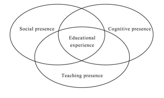
Presence can promote online learners' learning effectiveness in higher education, but in livestream teaching, the influential relationship between different types of presence and learning effectiveness is unclear. Therefore, based on the Community of Inquiry (CoI) Framework, we used structural equation, hierarchical regression, and the Bootstrap self-serving method to conduct a survey on college students participating in livestream teaching practice. The research findings revealed that livestream teaching substantially impacts learning effectiveness, with teaching presence, social presence, and cognitive presence all playing crucial roles. Notably, teaching presence has a significant positive influence on learning effectiveness through two key mediating factors: Social presence and cognitive presence. Consequently, three distinct mediating paths are identified. Among these three mediating paths, the most optimal route for teaching presence to enhance learning effectiveness is mediating cognitive presence. In conclusion, we recommend improving the livestream teaching environment, guiding learners toward active participation to promote a sense of embodiment, and elaborately designing livestream learning activities to improve interactivity. Finally, this paper offers evidence and insights for the improvement of livestream teaching in colleges, which will enhance learners' overall learning effectiveness.

References

[1]	Le, A., Satkunam, L. and Jaime, C.Y., Residents' Perceptions of a Novel Virtual Livestream Cadaveric Teaching Series for Musculoskeletal Anatomy Education. American Journal of Physical Medicine & Rehabilitation, 2023,102(12): e165–e168. https://doi.org/10.1097/PHM.0000000000002284 doi: 10.1097/PHM.0000000000002284
[2]	Hawdon, J.M. and Bernot, J.P., Teaching Parasitology Lab Remotely Using Livestreaming. The American Biology Teacher: Journal of the National Association of Biology Teachers, 2022, 84(5): 312–314. https://doi.org/10.1525/abt.2022.84.5.312 doi: 10.1525/abt.2022.84.5.312
[3]	UNESCO, Global education monitoring report, 2023: technology in education: a tool on whose terms? 2023.
[4]	Ma, L.P. and Bu, S.C., Is Synchronous Online Education Better than Asynchronous? An Empirical Study Based on Survey and Administration Data. Peking University Education Review, 2022, 20(3): 2-24+187.
[5]	Li, S., Huang, J.J. and Liu, S.Z., Analysis of Patterns and Characteristics of Teacher-Student Dialogue Interaction in Live Teaching. Modern Distance Education Research, 2022, 91–112.
[6]	Lin, X.F., Deng, C., Hu, Q. and Tsai, C.C., Chinese undergraduate students' perceptions of mobile learning: Conceptions, learning profiles, and approaches. Journal of Computer Assisted Learning, 2019, 35(3): 317–333. https://doi.org/10.1111/jcal.12333 doi: 10.1111/jcal.12333
[7]	Alqurashi, E., Technology Tools for Teaching and Learning in Real Time. 2019. Educational Technology and Resources for Synchronous Learning in Higher Education.
[8]	Wei, B.S., Analysis of Problems and Countermeasures in Open Education Livestream Teaching. Journal of Jilin Radio and TV University, 2018, 98-99+112.
[9]	Dunlap, J.C. and Lowenthal, P.R., Online educators' recommendations for teaching online: Crowdsourcing in action. Open Praxis, 2018, 10(1): 79–89. https://doi.org/10.5944/openpraxis.10.1.721 doi: 10.5944/openpraxis.10.1.721
[10]	Lin, X.F. and S.Q. Liu, Live Broadcast Teaching Strategies for Cultivating Higher-order Thinking Skills. Modern Educational Technology, 2019(03): 99–105.
[11]	Cui, X.P., Zhao, L., Su, W. and Lu, C.C., Research on the Structural Relationship and Effects of Influencing Factors of Live Learning Outcomes——From the Perspective of Interactive Distance Theory. e-Education Research, 2022, 63–70. https://doi.org/10.13811/j.cnki.eer.2022.01.008 doi: 10.13811/j.cnki.eer.2022.01.008
[12]	Kozan, K. and Richardson, J.C., Interrelationships Between and Among Social, Teaching, and Cognitive Presence. The Internet and higher education, 2014, 21: 68–73. https://doi.org/10.1016/j.iheduc.2013.10.007 doi: 10.1016/j.iheduc.2013.10.007
[13]	Wu, X.E., Chen, X.H. and Wu, J., On the Effects of Presence on Online Learning Performance. Modern Distance Education, 2017, 24–30. https://doi.org/10.13927/j.cnki.yuan.2017.0014 doi: 10.13927/j.cnki.yuan.2017.0014
[14]	Zhang, X.F., Shi, Y., Li, T., Guan, Y. and Cui, X., How Do Virtual AI Streamers Influence Viewers' Livestream Shopping Behavior? The Effects of Persuasive Factors and the Mediating Role of Arousal. Information Systems Frontiers, 2023, 1–32. https://doi.org/10.1007/s10796-023-10425-2 doi: 10.1007/s10796-023-10425-2
[15]	Garrison, D.R., Anderson, T. and Archer, W., Critical Inquiry in a Text-Based Environment: Computer Conferencing in Higher Education. The internet and higher education, 1999, 2(2-3): 87–105. https://doi.org/10.1016/S1096-7516(00)00016-6 doi: 10.1016/S1096-7516(00)00016-6
[16]	Garrison, D.R. and Arbaugh, J.B., Researching the community of inquiry framework: Review, issues, and future directions. Internet & Higher Education, 2007, 10(3): 157–172. https://doi.org/10.1016/j.iheduc.2007.04.001 doi: 10.1016/j.iheduc.2007.04.001
[17]	Garrison, D.R., Online Community of Inquiry Review: Social, Cognitive, and Teaching Presence Issues. Online Learning, 2007, 11(1). https://doi.org/10.24059/olj.v11i1.1737 doi: 10.24059/olj.v11i1.1737
[18]	Wan, L.Y., David, S. and Xie, K., Two Decades of Research on Community of Inquiry Framework: Retrospect and Prospect. Open Education Research, 2023, 26(06): 57–68. https://doi.org/10.13966/j.cnki.kfjyyj.2020.06.006 doi: 10.13966/j.cnki.kfjyyj.2020.06.006
[19]	Ma, Z.Q., Liu, Y.Q. and Kong, L.L., The Context and Inspiration of Theoretical and Empirical Research on the Community of Inquiry. Modern Distance Education Research, 2018, 39–48.
[20]	Goshtasbpour, F., Swinnerton, B. and Morris, N.P., Look Who's Talking: Exploring Instructors' Contributions to Massive Open Online Courses. British Journal of Educational Technology, 2020, 51(1): 228–244. https://doi.org/10.1111/bjet.12787 doi: 10.1111/bjet.12787
[21]	Shea, P. and Bidjerano, T., Community of inquiry as a theoretical framework to foster "epistemic engagement" and "cognitive presence" in online education. Computers & Education, 2009, 52(3): 543–553. https://doi.org/10.1016/j.compedu.2008.10.007 doi: 10.1016/j.compedu.2008.10.007
[22]	Hardin-Pierce, M., Hampton, D., Melander, S., Wheeler, K., Scott, L., Inman, D., et al., Faculty and Student Perspectives of a Graduate Online Delivery Model Supported by On-Campus Immersion. Clinical Nurse Specialist, 2020, 34(1): 23–29. https://doi.org/10.1097/NUR.0000000000000494 doi: 10.1097/NUR.0000000000000494
[23]	Bai, X.M., Ma, H.L. and Wu, H.M., Relationships among Teaching, Cognitive and Social Presence in a MOOC-based Blended Course. Open Education Research, 2016, 22(04): 71–78. https://doi.org/10.13966/j.cnki.kfjyyj.2016.04.009 doi: 10.13966/j.cnki.kfjyyj.2016.04.009
[24]	Rolim, V., Ferreira, R., Lins, R.D. and Gǎsević, D., A network-based analytic approach to uncovering the relationship between social and cognitive presences in communities of inquiry. The Internet and higher education, 2019, 42: 53–65. https://doi.org/10.1016/j.iheduc.2019.05.001 doi: 10.1016/j.iheduc.2019.05.001
[25]	Sun, K.T., Lin, Y.C. and Yu, C.J., A Study on Learning Effect among Different Learning Styles in a Web-Based Lab of Science at Elementary Schools. Computers & Education, 2008, 50(4): 1411–1422. https://doi.org/10.1016/j.compedu.2007.01.003 doi: 10.1016/j.compedu.2007.01.003
[26]	Cheung, W., Li, E.Y. and Yee, L.W., Multimedia learning system and its effect on self-efficacy in database modeling and design: an exploratory study. Computers & Education, 2003, 41(3): 249–270. https://doi.org/10.1016/S0360-1315(03)00048-4 doi: 10.1016/S0360-1315(03)00048-4
[27]	Latham, G.P. and Brown, T.C., The Effect of Learning vs. Outcome Goals on Self-Efficacy, Satisfaction and Performance in an MBA Program. Applied Psychology, 2006, 55(4): 606–623. https://doi.org/10.1111/j.1464-0597.2006.00246.x doi: 10.1111/j.1464-0597.2006.00246.x
[28]	Sung, Y.T., Chang, K.E. and Liu, T.C., The effects of integrating mobile devices with teaching and learning on students' learning performance. Pergamon, 2016, 94: 252–275. https://doi.org/10.1016/j.compedu.2015.11.008 doi: 10.1016/j.compedu.2015.11.008
[29]	Zhong, B.C. and Xia, L.Y., Effects of new coopetition designs on learning performance in robotics education. Journal of Computer Assisted Learning, 2021, 38(1): 223–236. https://doi.org/10.1111/jcal.12606 doi: 10.1111/jcal.12606
[30]	Fung, C.J.L. and Lang, Q.C., Modelling relationships between students' academic achievement and community of inquiry in an online learning environment for a blended course. Australasian Journal of Educational Technology, 2016, 32(4). https://doi.org/10.14742/ajet.2500 doi: 10.14742/ajet.2500
[31]	Garrison, D.R., Clevelandinnes, M. and Fung, T.S., Exploring causal relationships among teaching, cognitive and social presence: Student perceptions of the community of inquiry framework. Internet & Higher Education, 2010, 13(1): 31–36. https://doi.org/10.1016/j.iheduc.2009.10.002 doi: 10.1016/j.iheduc.2009.10.002
[32]	Guoshuai, L., Qiuju, Z., Caijie, L.V., Yating, S. and Jiacai, W., Construction of a Chinese Version of the Community of Inquiry Measurement Instrument. Open Education Research, 2018, 24(03): 68–76. https://doi.org/10.13966/j.cnki.kfjyyj.2018.03.008 doi: 10.13966/j.cnki.kfjyyj.2018.03.008
[33]	Aldhahi, M.I., Alqahtani, A.S., Baattaiah, B.A. and Al-Mohammed, H.I., Exploring the relationship between students' learning satisfaction and self-efficacy during the emergency transition to remote learning amid the coronavirus pandemic: A cross-sectional study. Education and information technologies, 2022, 27(1): 1323–1340. https://doi.org/10.1007/s10639-021-10644-7 doi: 10.1007/s10639-021-10644-7
[34]	Thomas, L.J., Parsons, M. and Whitcombe, D., Assessment in Smart Learning Environments: Psychological Factors Affecting Perceived Learning. Computers in Human Behavior, 2018, 95: 197–207. https://doi.org/10.1016/j.chb.2018.11.037 doi: 10.1016/j.chb.2018.11.037
[35]	Wen, Z.L. and Ye, B.J., Analyses of Mediating Effects: The Development of Methods and Models. Advances in Psychological ence, 2014, 22(5): 731–745. https://doi.org/10.3724/SP.J.1042.2014.00731 doi: 10.3724/SP.J.1042.2014.00731
[36]	Li, S.W., Luo, J.L. and Ge, Y.Q., Effects of Big Data Analysis Capability on Breakthrough Product Innovation. Journal of Management Science, 2021, 3–15.
[37]	Dixson, M.D., Creating effective student engagement in online courses: What do students find engaging? Journal of the Scholarship of Teaching and Learning, 2010, 10(2): 1–13.
[38]	Contreras, C.P., Picazo, D., Cordero-Hidalgo, A. and Chaparro-Medina, P.M., Challenges of virtual education during the Covid-19 pandemic: Experiences of mexican university professors and students. International Journal of Learning, Teaching and Educational Research, 2021, 20(3): 188204. https://doi.org/10.26803/ijlter.20.3.12 doi: 10.26803/ijlter.20.3.12
[39]	Kwiatkowska, W. and Winiewska-Nogaj, L., Motives, benefits and difficulties in online collaborative learning versus the field of study. An empirical research project concerning Polish students. e-mentor, 2021, 90(3): 11–21. https://doi.org/10.15219/em90.1518 doi: 10.15219/em90.1518
[40]	Zhang, W.W., Zhu, J. and Jiang, X., Research on the Impact of Social Learning on the Knowledge Contribution Behavior of Different Types of Users in Professional Virtual Communities. Information and Documentation Services, 2021, 42(5): 94–103.
[41]	Li, Y.F., Zhou, X.Z. and Yang, X.H., The Optimization Design of Online Open Courses for Subjects Needs. Modern Educational Technology, 2022,104–110.
[42]	Ghazali, A.F., Othman, A.K., Sokman, Y., Zainuddi, N.A., Suhaimi, A., Mokhtar, N.A. et al., Investigating Social Cognitive Theory in Online Distance and Learning for Decision Support: The Case for Community of Inquiry. International Journal of Asian Social Science, 2021, 11(11): 522–538.
[43]	Yang, S.J., How to Ensure the Teaching Quality of Online Live Courses——Taking the Learning Environment and Learning Content Design of Online Live Courses during the Epidemic as an Example. Modern Educational Technology, 2023,112–118.
[44]	Valentini, M. and Guarnacci, S., Embodied cognition, effective learning and physical activity as a shared feature: Systematic review. Universidad de Alicante. Área de Educación Física y Deporte, 2021, 16(2): S539–S552. https://doi.org/10.14198/JHSE.2021.16.PROC2.38 doi: 10.14198/JHSE.2021.16.PROC2.38
[45]	Guo, S.Q., Gao, H.Y. and Hua, X.Y., Theoretical Research on Design of "Internet +" Unit Teaching Mode. e-Education Research, 2022, 43(06): 91-103+112. https://doi.org/10.13811/j.cnki.eer.2022.06.014 doi: 10.13811/j.cnki.eer.2022.06.014
[46]	Cui, X.P., et al., Visualization Analysis of Online Learning Activity Design Research in China. Journal of Longdong University, 2023, 32(4): 135–139.

Author's biography Prof. Xiangping Cui, Lanzhou, China, Doctoral degree in educational technology, Northwest Normal University, Lanzhou, China, 2014. Research field: Online education and Smart education. She was a visiting scholar at the Ohio State University (2019). She is now a Professor at the Institute of Higher Education of Lanzhou University in Lanzhou, China. In recent years, she has published more than 40 papers and 6 textbooks and monographs. Now her main research interest is online education and smart education. Dr. Cui has won the Google Teaching Award in 2020 and won the Silver Award of "MOOC China Cup" quality online education course Teaching Organization in 2019.She can be contacted at email:cuixp@lzu.edu.cn; Mr Jiangming Qian is s a master's student at Institute of Higher Education of Lanzhou University in Lanzhou, China. He is specializing in online education. He's the author of the article "The Influence of Blockly Visual Programming on College Students' Innovative Ability" (Journal of Open Learning, 2023). He can be contacted at email: qianjm21@lzu.edu.cn; Soheila Garshasbi, a committed PhD candidate at the University of Wollongong's School of Computing and Information Technology, is acknowledged for her meaningful contributions to educational technology research, particularly in the STEM domain. With a background in TEFL (Teaching English as a Foreign Language) and a decade of experience as an ESL/EFL lecturer, her expertise spans education technology, problem-solving, academic self-concept, and cultivating a teamwork attitude in STEM education and language learning. Leveraging cutting-edge metaheuristic AI/ML-enabled modelling and optimization algorithms, Garshasbi's research aims to enhance collaborative language learning by improving group dynamics within STEM contexts. She can be contacted at email: sg908@uowmail.edu.au; Ms Susan Zhang is a final year Ph.D. student in Information Technology at UOW with a laser focus on Educational Key Opinion Leader at the intersection of E-learning Technology and Pedagogy Transformation. She holds dual Bachelor's degrees in Computer Science and Software Engineering from Zhengzhou University, China and the University of Wollongong(UOW), Australia, and a Master of Information Communication Technology majoring in Enterprise Networking. Previously, Ms Zhang's career has taken her to dizzying heights in Australia, China and the United Kingdom, where she has worked at Google, ByteDance (TikTok) and Amazon. Ms Zhang is a published author, a dynamic inspirational speaker at TEDx, IEEE and many other top industries conferences. Her curiosity, passion and strong belief in Educational change drove her pivot from Tech Industry to Academic educational research, with the hope and goal to make a contribution in this area. She can be contacted at email: xiaochen@uow.edu.au; Dr. Geng Sun is an adjunct professor at the School of Engineering, Chongqing College of Humanities, Science and Technology, China and the director of Vermilion Cloud, Australia. He obtained his PhD degree from the School of Computing and Information Technology, University of Wollongong, Australia in 2018 with Examiners' commendation for outstanding thesis. His current research interests and focus are education in the Web3 era, AI in education, intelligent tutoring systems, and computational intelligence in adaptive learning. He has published more than 50 papers in leading journals and conferences, with attracting more than 600 citations. He can be contacted at email: gsun@vermilioncloud.com.au; Juan Wang, Xuzhou, China, Doctoral degree in educational technology, Northwest Normal University, Lanzhou, China, 2013. Research field: Smart Education, Blended Learning, STEAM Education, and Education Big Data. She was a visiting scholar at Missouri University (2013) and Hong Kong University (2014). She is a professor at the School of Smart Education at Jiangsu Normal University, Xuzhou, China. In recent years, She has published over 70 papers in authoritative professional journals, led 19 national and provincial projects, and published 5 academic works, and received multiple honours. She can be contacted at email: wangjuan@jsnu.edu.cn; Prof. Jun Shen is an active researcher in multi-disciplines where computational intelligence, cloud, IoT, and learning technologies are applied to solving real-life problems. Jun Shen was awarded a Ph.D. in 2001 at Southeast University, China. He held positions at Swinburne University of Technology and the University of South Australia before 2006. Currently, he is an Associate Professor in the School of Computing and Information Technology at UOW, NSW, Australia. He is a senior member of IEEE, ACM and ACS and has been engaged in many funded projects (supported by ARC/CRC, NSFC, UGPN, etc). He published more than 250 papers in journals and conferences in CS/IT areas. He has been Editor, PC Chair, Guest Editor, and PC Member for numerous journals and conferences published by IEEE, ACM, Elsevier, and Springer. He can be contacted at email: jshen@uow.edu.au; Dr. Lin Yue is currently the Course Director of Master of Business Analytics and Lecturer in the Department of Actuarial Studies and Business Analytics at Macquarie Business School. She holds a PhD in Information Systems from UNSW, a Master's degree in Computer Science from Trinity College Dublin and a Bachelor's degree in Computer Science (Honours) with First Class Honours. Lin has published several papers on digital enablement, digital innovations and business analytics applications in leading information systems (IS) journals and conferences. Lin is also the associate editor of several ABDC A* journals. She also has a strong background in financial trading as a financial trader. Combining her robust analytical prowess and effective leadership skills, with a background in computer science and business analytics, enables her to collaborate seamlessly across various disciplines and attain high levels of research success with a focus on practical applications. She can be contacted at email: lin.yue@mq.edu.au; Yewen Lyu obtained Master's degree in Arts and Cultural Management at the University of Melbourne. She is specialized in cultural industries. Her research is centered around key aspects such as arts education, arts marketing, cultural dynamics, and the art market economy. She can be contacted at email: yewenl@student.unimelb.edu.au

Reader Comments

Your name:*

Email:*
© 2024 the Author(s), licensee AIMS Press. This is an open access article distributed under the terms of the Creative Commons Attribution License (http://creativecommons.org/licenses/by/4.0)