There is an absence of valid and specific psychometric tools to assess TikTok addiction. Considering that the use of TikTok is increasing rapidly and the fact that TikTok addiction may be a different form of social media addiction, there is an urge for a valid tool to measure TikTok addiction.
To develop and validate a tool to measure TikTok addiction.
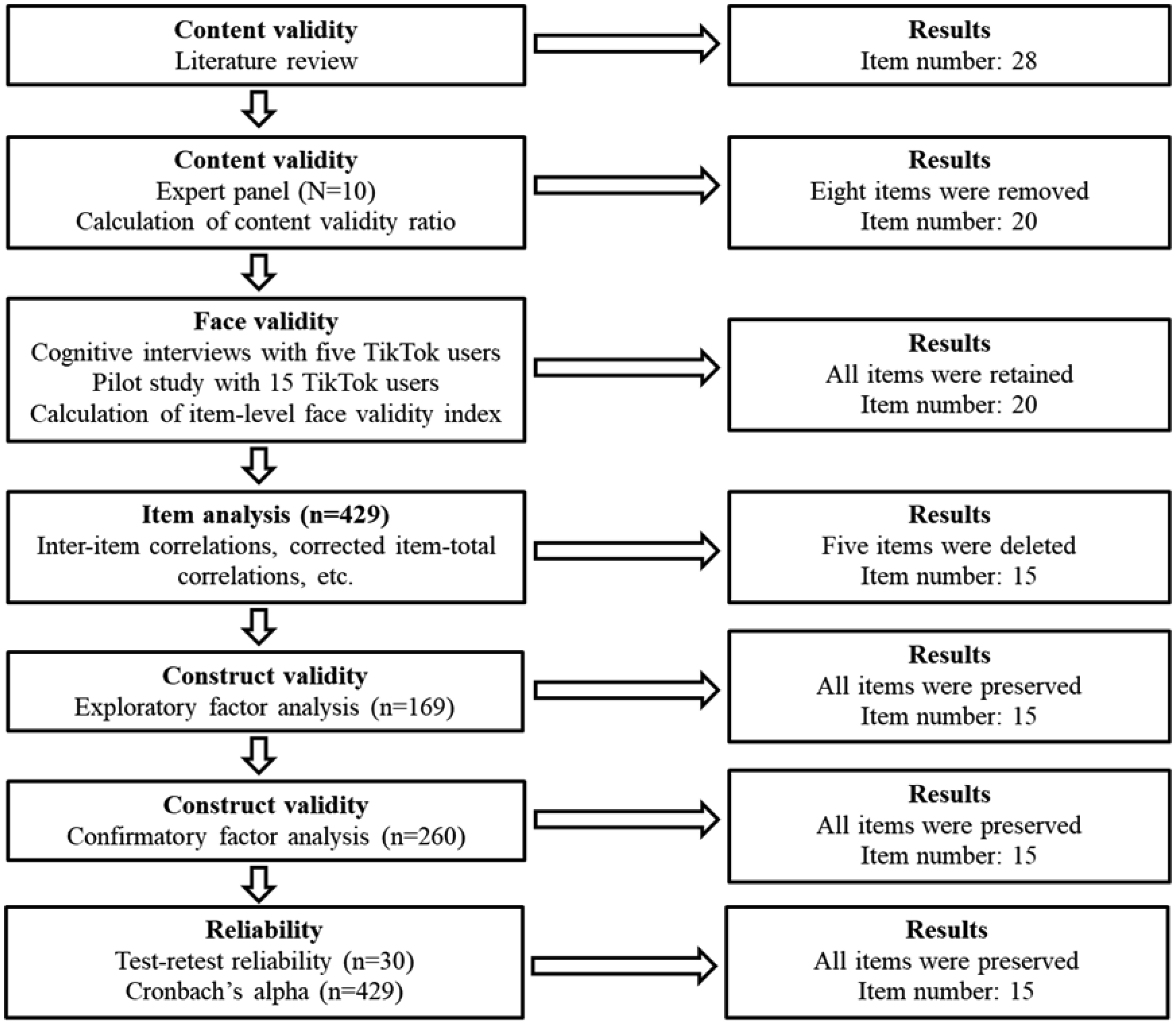
First, we performed an extensive literature review to create a pool of items to measure TikTok addiction. Then, we employed a panel of experts from different backgrounds to examine the content validity of the initial set of items. We examined face validity by performing cognitive interviews with TikTok users and calculating the item-level face validity index. Our study population included 429 adults who have been TikTok users for at least the last 12 months. We employed exploratory and confirmatory factor analysis to examine the construct validity of the TikTok Addiction Scale (TTAS). We examined the concurrent validity by using the Bergen Social Media Addiction Scale (BSMAS), the Patient Health Questionnaire-4 (PHQ-4), and the Big Five Inventory-10 (BFI-10). We used Cronbach's alpha, McDonald's Omega, Cohen's kappa, and intraclass correlation coefficient to examine reliability.
We found that the TTAS is a six-factor 15-item scale with robust psychometric properties. Factor analysis revealed a six-factor structure, (1) salience, (2) mood modification, (3) tolerance, (4) withdrawal symptoms, (5) conflict, and (6) relapse, which accounted for 80.70% of the total variance. The concurrent validity of the TTAS was excellent since we found significant correlations between TTAS and BSMAS, PHQ-4, and BFI-10. Cronbach's alpha and McDonald's Omega for the TTAS were 0.911 and 0.914, respectively.
The TTAS appears to be a short, easy-to-use, and valid scale to measure TikTok addiction. Considering the limitations of our study, we recommend the translation and validation of the TTAS in other languages and populations to further examine the validity of the scale.
Citation: Petros Galanis, Aglaia Katsiroumpa, Ioannis Moisoglou, Olympia Konstantakopoulou. The TikTok Addiction Scale: Development and validation[J]. AIMS Public Health, 2024, 11(4): 1172-1197. doi: 10.3934/publichealth.2024061
There is an absence of valid and specific psychometric tools to assess TikTok addiction. Considering that the use of TikTok is increasing rapidly and the fact that TikTok addiction may be a different form of social media addiction, there is an urge for a valid tool to measure TikTok addiction.
To develop and validate a tool to measure TikTok addiction.
First, we performed an extensive literature review to create a pool of items to measure TikTok addiction. Then, we employed a panel of experts from different backgrounds to examine the content validity of the initial set of items. We examined face validity by performing cognitive interviews with TikTok users and calculating the item-level face validity index. Our study population included 429 adults who have been TikTok users for at least the last 12 months. We employed exploratory and confirmatory factor analysis to examine the construct validity of the TikTok Addiction Scale (TTAS). We examined the concurrent validity by using the Bergen Social Media Addiction Scale (BSMAS), the Patient Health Questionnaire-4 (PHQ-4), and the Big Five Inventory-10 (BFI-10). We used Cronbach's alpha, McDonald's Omega, Cohen's kappa, and intraclass correlation coefficient to examine reliability.
We found that the TTAS is a six-factor 15-item scale with robust psychometric properties. Factor analysis revealed a six-factor structure, (1) salience, (2) mood modification, (3) tolerance, (4) withdrawal symptoms, (5) conflict, and (6) relapse, which accounted for 80.70% of the total variance. The concurrent validity of the TTAS was excellent since we found significant correlations between TTAS and BSMAS, PHQ-4, and BFI-10. Cronbach's alpha and McDonald's Omega for the TTAS were 0.911 and 0.914, respectively.
The TTAS appears to be a short, easy-to-use, and valid scale to measure TikTok addiction. Considering the limitations of our study, we recommend the translation and validation of the TTAS in other languages and populations to further examine the validity of the scale.

| [1] | StatistaStatista, Social Media & User-Generated Content, 2024 (2024). Available from: https://www.statista.com/statistics/278414/number-of-worldwide-social-network-users/ |
| [2] |
Meng SQ, Cheng JL, Li YY, et al. (2022) Global prevalence of digital addiction in general population: A systematic review and meta-analysis. Clin Psychol Rev 92: 102128. https://doi.org/10.1016/j.cpr.2022.102128 
|
| [3] |
Cheng C, Lau Y, Chan L, et al. (2021) Prevalence of social media addiction across 32 nations: Meta-analysis with subgroup analysis of classification schemes and cultural values. Addict Behav 117: 106845. https://doi.org/10.1016/j.addbeh.2021.106845
|
| [4] |
Arrivillaga C, Rey L, Extremera N (2022) A mediated path from emotional intelligence to problematic social media use in adolescents: The serial mediation of perceived stress and depressive symptoms. Addict Behav 124: 107095. https://doi.org/10.1016/j.addbeh.2021.107095
|
| [5] |
Bányai F, Zsila Á, Király O, et al. (2017) Problematic Social Media Use: Results from a Large-Scale Nationally Representative Adolescent Sample. PLoS ONE 12: e0169839. https://doi.org/10.1371/journal.pone.0169839
|
| [6] |
Sindermann C, Elhai JD, Montag C (2020) Predicting tendencies towards the disordered use of Facebook's social media platforms: On the role of personality, impulsivity, and social anxiety. Psychiatry Res 285: 112793. https://doi.org/10.1016/j.psychres.2020.112793
|
| [7] |
Keles B, McCrae N, Grealish A (2020) A systematic review: The influence of social media on depression, anxiety and psychological distress in adolescents. Int J Adolesc Youth 25: 79-93. https://doi.org/10.1080/02673843.2019.1590851
|
| [8] |
Kuss D, Griffiths M, Karila L, et al. (2014) Internet Addiction: A Systematic Review of Epidemiological Research for the Last Decade. CPD 20: 4026-4052. https://doi.org/10.2174/13816128113199990617
|
| [9] |
Xanidis N, Brignell CM (2016) The association between the use of social network sites, sleep quality and cognitive function during the day. Comput Human Behav 55: 121-126. https://doi.org/10.1016/j.chb.2015.09.004
|
| [10] |
Huang C (2022) A meta-analysis of the problematic social media use and mental health. Int J Soc Psychiatry 68: 12-33. https://doi.org/10.1177/0020764020978434
|
| [11] |
Shannon H, Bush K, Villeneuve PJ, et al. (2022) Problematic social media use in adolescents and young adults: Systematic review and meta-analysis. JMIR Ment Health 9: e33450. https://doi.org/10.2196/33450
|
| [12] |
Hong Y, Rong X, Liu W (2024) Construction of influencing factor segmentation and intelligent prediction model of college students' cell phone addiction model based on machine learning algorithm. Heliyon 10: e29245. https://doi.org/10.1016/j.heliyon.2024.e29245
|
| [13] | DatareportalDatareportal, Global social media statistics, 2024 (2024). Available from: https://datareportal.com/social-media-users |
| [14] | HumbleGreeks & social media research: An up-to-date Whitepaper for the Greek market, 2024 (2024). Available from: https://humble.gr/blog/insights/humble-research/ |
| [15] |
Montag C, Yang H, Elhai JD (2021) On the psychology of TikTok use: A first glimpse from empirical findings. Front Public Health 9: 641673. https://doi.org/10.3389/fpubh.2021.641673
|
| [16] |
Lodice R, Papapicco C (2021) To be a TikToker in COVID-19 era: An experience of social influence. Online J Commun Medi 11: e202103. https://doi.org/10.30935/ojcmt/9615
|
| [17] |
Smith T, Short A (2022) Needs affordance as a key factor in likelihood of problematic social media use: Validation, latent Profile analysis and comparison of TikTok and Facebook problematic use measures. Addict Behav 129: 107259. https://doi.org/10.1016/j.addbeh.2022.107259
|
| [18] |
Casale S, Rugai L, Fioravanti G (2018) Exploring the role of positive metacognitions in explaining the association between the fear of missing out and social media addiction. Addict Behav 85: 83-87. https://doi.org/10.1016/j.addbeh.2018.05.020
|
| [19] |
Tarafdar M, Maier C, Laumer S, et al. (2020) Explaining the link between technostress and technology addiction for social networking sites: A study of distraction as a coping behavior. Inf Syst J 30: 96-124. https://doi.org/10.1111/isj.12253
|
| [20] |
Iram, Aggarwal H (2020) Time series analysis of pubg and tiktok applications using sentiments obtained from social media-twitter. Adv Math, Sci J 9: 4047-4057. https://doi.org/10.37418/amsj.9.6.86
|
| [21] |
Zhang X, Wu Y, Liu S (2019) Exploring short-form video application addiction: Socio-technical and attachment perspectives. Telemat Inform 42: 101243. https://doi.org/10.1016/j.tele.2019.101243
|
| [22] |
Lu L, Liu M, Ge B, et al. (2022) Adolescent addiction to short video applications in the mobile internet era. Front Psychol 13: 893599. https://doi.org/10.3389/fpsyg.2022.893599
|
| [23] |
Qin Y, Musetti A, Omar B (2023) Flow experience is a key factor in the likelihood of adolescents' problematic TikTok use: The moderating role of active parental mediation. IJERPH 20: 2089. https://doi.org/10.3390/ijerph20032089
|
| [24] |
Montag C, Lachmann B, Herrlich M, et al. (2019) Addictive features of social media/messenger platforms and freemium games against the background of psychological and economic theories. IJERPH 16: 2612. https://doi.org/10.3390/ijerph16142612
|
| [25] | Burhan R, Moradzadeh J (2020) Neurotransmitter Dopamine (DA) and its role in the development of social media addiction. J Neurol Neurophysiol 11: 1-2. |
| [26] |
Su C, Zhou H, Gong L, et al. (2021) Viewing personalized video clips recommended by TikTok activates default mode network and ventral tegmental area. NeuroImage 237: 118136. https://doi.org/10.1016/j.neuroimage.2021.118136
|
| [27] |
Varona MN, Muela A, Machimbarrena JM (2022) Problematic use or addiction? A scoping review on conceptual and operational definitions of negative social networking sites use in adolescents. Addict Behav 134: 107400. https://doi.org/10.1016/j.addbeh.2022.107400
|
| [28] |
Andreassen CS, Torsheim T, Brunborg GS, et al. (2012) Development of a facebook addiction scale. Psychol Rep 110: 501-517. https://doi.org/10.2466/02.09.18.PR0.110.2.501-517
|
| [29] |
Andreassen CS, Billieux J, Griffiths MD, et al. (2016) The relationship between addictive use of social media and video games and symptoms of psychiatric disorders: A large-scale cross-sectional study. Psychol Addict Behav 30: 252-262. https://doi.org/10.1037/adb0000160
|
| [30] |
Van Den Eijnden RJJM, Lemmens JS, Valkenburg PM (2016) The social media disorder scale. Comput Human Behav 61: 478-487. https://doi.org/10.1016/j.chb.2016.03.038
|
| [31] |
Elphinston RA, Noller P (2011) Time to face it! Facebook intrusion and the implications for romantic jealousy and relationship satisfaction. Cyberpsychol Behav Soc Netw 14: 631-635. https://doi.org/10.1089/cyber.2010.0318
|
| [32] |
Caplan SE (2010) Theory and measurement of generalized problematic Internet use: A two-step approach. Comput Human Behav 26: 1089-1097. https://doi.org/10.1016/j.chb.2010.03.012
|
| [33] |
Young KS (1998) Internet addiction: The emergence of a new clinical disorder. Cyberpsychol Behav 1: 237-244. https://doi.org/10.1089/cpb.1998.1.237
|
| [34] |
Dadiotis A, Bacopoulou F, Kokka I, et al. (2021) Validation of the Greek version of the Bergen social media addiction scale in undergraduate students. EMBnet J 26: e975. https://doi.org/10.14806/ej.26.1.975
|
| [35] |
Floros G, Siomos K (2012) Patterns of choices on video game genres and internet addiction. Cyberpsychol Behav Soc Netw 15: 417-424. https://doi.org/10.1089/cyber.2012.0064
|
| [36] |
Kokka I, Mourikis I, Michou M, et al. (2021) Validation of the Greek version of social media disorder scale. GeNeDis 2020 . Cham: Springer International Publishing 107-116. https://doi.org/10.1007/978-3-030-78775-2_13
|
| [37] |
Zhu J, Ma Y, Xia G, et al. (2024) Self-perception evolution among university student TikTok users: evidence from China. Front Psychol 14: 1217014. https://doi.org/10.3389/fpsyg.2023.1217014
|
| [38] |
Alhabash S, Smischney TM, Suneja A, et al. (2024) So similar, yet so different: How motivations to use Facebook, Instagram, Twitter, and TikTok predict problematic use and use continuance intentions. Sage Open 14: 21582440241255426. https://doi.org/10.1177/21582440241255426
|
| [39] |
Hendrikse C, Limniou M (2024) The use of Instagram and TikTok in relation to problematic use and well-being. J Technol Behav Sci 9: 1-12. https://doi.org/10.1007/s41347-024-00399-6
|
| [40] | Yang Y, Adnan H, Sarmiti N (2023) The relationship between anxiety and TikTok addiction among university students in China: Mediated by escapism and use intensity. Int J Media Inf Lit 8. https://doi.org/10.13187/ijmil.2023.2.458 |
| [41] |
Rogowska AM, Cincio A (2024) Procrastination mediates the relationship between problematic TikTok Use and depression among young adults. JCM 13: 1247. https://doi.org/10.3390/jcm13051247
|
| [42] |
Pontes HM, Schivinski B, Sindermann C, et al. (2021) Measurement and conceptualization of gaming disorder according to the World Health Organization framework: The development of the gaming disorder test. Int J Ment Health Addiction 19: 508-528. https://doi.org/10.1007/s11469-019-00088-z
|
| [43] |
Montag C, Markett S (2024) Depressive inclinations mediate the association between personality (neuroticism/conscientiousness) and TikTok Use Disorder tendencies. BMC Psychol 12: 81. https://doi.org/10.1186/s40359-024-01541-y
|
| [44] |
McCoach D, Gable R, Madura J (2013) Review of the steps for designing an instrument. Instrument development in the affective domain . New York: Springer 277-284. https://doi.org/10.1007/978-1-4614-7135-6_8
|
| [45] |
Bekalu MA, Sato T, Viswanath K (2023) Conceptualizing and measuring social media use in health and well-being studies: Systematic review. J Med Internet Res 25: e43191. https://doi.org/10.2196/43191
|
| [46] |
Darvesh N, Radhakrishnan A, Lachance CC, et al. (2020) Exploring the prevalence of gaming disorder and internet gaming disorder: A rapid scoping review. Syst Rev 9: 68. https://doi.org/10.1186/s13643-020-01329-2
|
| [47] |
Pan YC, Chiu YC, Lin YH (2020) Systematic review and meta-analysis of epidemiology of internet addiction. Neurosci Biobehav Rev 118: 612-622. https://doi.org/10.1016/j.neubiorev.2020.08.013
|
| [48] | Brown R (1993) Some contributions of the study of gambling to the study of other addictions. Gambling Behaviour and Problem Gambling . Reno: University of Nevada Press 241-272. |
| [49] |
Griffiths M (1996) Nicotine, tobacco and addiction. Nature 384: 18. https://doi.org/10.1038/384018a0
|
| [50] | Griffiths M (2005) A ‘components’ model of addiction within a biopsychosocial framework. J Subst Abuse 10: 191-197. https://doi.org/10.1080/14659890500114359 |
| [51] | WHOInternational classification of diseases 11th revision, 2024 (2024). Available from: https://icd.who.int/en |
| [52] |
Ayre C, Scally AJ (2014) Critical values for Lawshe's content validity ratio: Revisiting the original methods of calculation. Meas Eval Counsel Dev 47: 79-86. https://doi.org/10.1177/0748175613513808
|
| [53] |
Meadows K (2021) Cognitive interviewing methodologies. Clin Nurs Res 30: 375-379. https://doi.org/10.1177/10547738211014099
|
| [54] |
Yusoff MSB (2019) ABC of response process validation and face validity index calculation. EIMJ 11: 55-61. https://doi.org/10.21315/eimj2019.11.3.6
|
| [55] | Costello AB, Osborne J (2005) Best practices in exploratory factor analysis: Four recommendations for getting the most from your analysis. Pract Assess Res Eval 10: 1-9. |
| [56] |
DeVon HA, Block ME, Moyle-Wright P, et al. (2007) A psychometric toolbox for testing validity and reliability. J Nurs Scholarsh 39: 155-164. https://doi.org/10.1111/j.1547-5069.2007.00161.x
|
| [57] | De Vaus D (2004) Surveys in social research. London: Routledge 180-200. |
| [58] |
Yusoff MSB, Arifin WN, Hadie SNH (2021) ABC of questionnaire development and validation for survey research. EIMJ 13: 97-108. https://doi.org/10.21315/eimj2021.13.1.10
|
| [59] | Hair J, Black W, Babin B, et al. (2017) Multivariate data analysis. New Jersey: Prentice Hall 45-55. |
| [60] |
De Winter JCF, Dodou D, Wieringa PA (2009) Exploratory factor analysis with small sample sizes. Multivariate Behav Res 44: 147-181. https://doi.org/10.1080/00273170902794206
|
| [61] | Klein R (2016) Principles and practice of structural equation modelling. New York: Guilford Press 188-210. |
| [62] |
Bland JM, Altman DG (1997) Statistics notes: Cronbach's alpha. BMJ 314: 572-572. https://doi.org/10.1136/bmj.314.7080.572
|
| [63] | Brown T (2015) Confirmatory factor analysis for applied research. New York: The Guilford Press 72-87. |
| [64] |
Hu L, Bentler PM (1998) Fit indices in covariance structure modeling: Sensitivity to underparameterized model misspecification. Psychol Methods 3: 424-453. https://doi.org/10.1037/1082-989X.3.4.424
|
| [65] |
Baumgartner H, Homburg C (1996) Applications of structural equation modeling in marketing and consumer research: A review. Int J Res Mark 13: 139-161. https://doi.org/10.1016/0167-8116(95)00038-0
|
| [66] | Kroenke K, Spitzer RL, Williams JBW, et al. (2009) An ultra-brief screening scale for anxiety and depression: The PHQ-4. Psychosomatics 50: 613-621. https://doi.org/10.1176/appi.psy.50.6.613 |
| [67] |
Rammstedt B, John OP (2007) Measuring personality in one minute or less: A 10-item short version of the Big Five Inventory in English and German. J Res Pers 41: 203-212. https://doi.org/10.1016/j.jrp.2006.02.001
|
| [68] |
Copez-Lonzoy A, Vallejos-Flores M, Capa-Luque W, et al. (2023) Adaptation of the Bergen Social Media Addiction Scale (BSMAS) in Spanish. Acta Psychol (Amst) 241: 104072. https://doi.org/10.1016/j.actpsy.2023.104072
|
| [69] | Brailovskaia J, Margraf J (2022) Addictive social media use during Covid-19 outbreak: Validation of the Bergen Social Media Addiction Scale (BSMAS) and investigation of protective factors in nine countries. Curr Psychol 1–19. https://doi.org/10.1007/s12144-022-03182-z |
| [70] |
Shin NY (2022) Psychometric properties of the bergen social media addiction scale in Korean young adults. Psychiatry Investig 19: 356-361. https://doi.org/10.30773/pi.2021.0294
|
| [71] |
Žmavc M, Šorgo A, Gabrovec B, et al. (2022) The protective role of resilience in the development of social media addiction in tertiary students and psychometric properties of the Slovenian Bergen Social Media Addiction Scale (BSMAS). Int J Environ Res Public Health 19: 13178. https://doi.org/10.3390/ijerph192013178
|
| [72] |
Rouleau RD, Beauregard C, Beaudry V (2023) A rise in social media use in adolescents during the COVID-19 pandemic: the French validation of the Bergen Social Media Addiction Scale in a Canadian cohort. BMC Psychol 11: 92. https://doi.org/10.1186/s40359-023-01141-2
|
| [73] |
Cunningham S, Hudson CC, Harkness K (2021) Social media and depression symptoms: A meta-analysis. Res Child Adolesc Psychopathol 49: 241-253. https://doi.org/10.1007/s10802-020-00715-7
|
| [74] |
Hussain Z, Wegmann E, Yang H, et al. (2020) Social networks use disorder and associations with depression and anxiety symptoms: A systematic review of recent research in China. Front Psychol 11: 211. https://doi.org/10.3389/fpsyg.2020.00211
|
| [75] |
Caro-Fuentes S, Sanabria-Mazo JP (2024) A systematic review of the psychometric properties of the patient Health Questionnaire-4 in clinical and nonclinical populations. J Acad Consult Liaison Psychiatry 65: 178-194. https://doi.org/10.1016/j.jaclp.2023.11.685
|
| [76] |
Meidl V, Dallmann P, Leonhart R, et al. (2024) Validation of the patient health Questionnaire-4 for longitudinal mental health evaluation in elite Para athletes. PM R 16: 141-149. https://doi.org/10.1002/pmrj.13011
|
| [77] |
Rodríguez-Muñoz M de la F, Ruiz-Segovia N, Soto-Balbuena C, et al. (2020) The psychometric properties of the patient health Questionnaire-4 for pregnant women. Int J Environ Res Public Health 17: 7583. https://doi.org/10.3390/ijerph17207583
|
| [78] |
Tan YK, Siau CS, Ibrahim N, et al. (2024) Validation of the Malay version of the Patient Health Questionnaire-4 (PHQ-4) among Malaysian undergraduates. Asian J Psychiatr 99: 104134. https://doi.org/10.1016/j.ajp.2024.104134
|
| [79] |
Karekla M, Pilipenko N, Feldman J (2012) Patient health questionnaire: Greek language validation and subscale factor structure. Compr Psychiatry 53: 1217-1226. https://doi.org/10.1016/j.comppsych.2012.05.008
|
| [80] |
Correa T, Hinsley AW, De Zúñiga HG (2010) Who interacts on the Web?: The intersection of users' personality and social media use. Comput Human Behav 26: 247-253. https://doi.org/10.1016/j.chb.2009.09.003
|
| [81] |
Kuss DJ, Griffiths MD (2011) Online social networking and addiction—A review of the psychological literature. IJERPH 8: 3528-3552. https://doi.org/10.3390/ijerph8093528
|
| [82] |
Wilson K, Fornasier S, White KM (2010) Psychological predictors of young adults' use of social networking sites. Cyberpsychol Behav Soc Netw 13: 173-177. https://doi.org/10.1089/cyber.2009.0094
|
| [83] |
Kunnel John R, Xavier B, Waldmeier A, et al. (2019) Psychometric evaluation of the BFI-10 and the NEO-FFI-3 in Indian adolescents. Front Psychol 10: 1057. https://doi.org/10.3389/fpsyg.2019.01057
|
| [84] |
Costa Mastrascusa R, De Oliveira Fenili Antunes ML, De Albuquerque NS, et al. (2023) Evaluating the complete (44-item), short (20-item) and ultra-short (10-item) versions of the Big Five Inventory (BFI) in the Brazilian population. Sci Rep 13: 7372. https://doi.org/10.1038/s41598-023-34504-1
|
| [85] |
Balgiu BA (2018) The psychometric properties of the Big Five inventory-10 (BFI-10) including correlations with subjective and psychological well-being. GJPR 8: 61-69. https://doi.org/10.18844/gjpr.v8i2.3434
|
| [86] |
Soto CJ, John OP (2017) The next Big Five Inventory (BFI-2): Developing and assessing a hierarchical model with 15 facets to enhance bandwidth, fidelity, and predictive power. J Pers Soc Psychol 113: 117-143. https://doi.org/10.1037/pspp0000096
|
| [87] | World Medical Association.World medical association declaration of Helsinki: Ethical principles for medical research involving human subjects. JAMA (2013) 310: 2191. https://doi.org/10.1001/jama.2013.281053 |
 publichealth-11-04-061-s001.pdf publichealth-11-04-061-s001.pdf |
 |

Figures(2) / Tables(4)

Petros Galanis, Aglaia Katsiroumpa, Ioannis Moisoglou, Olympia Konstantakopoulou. The TikTok Addiction Scale: Development and validation[J]. AIMS Public Health, 2024, 11(4): 1172-1197. doi: 10.3934/publichealth.2024061


 DownLoad: