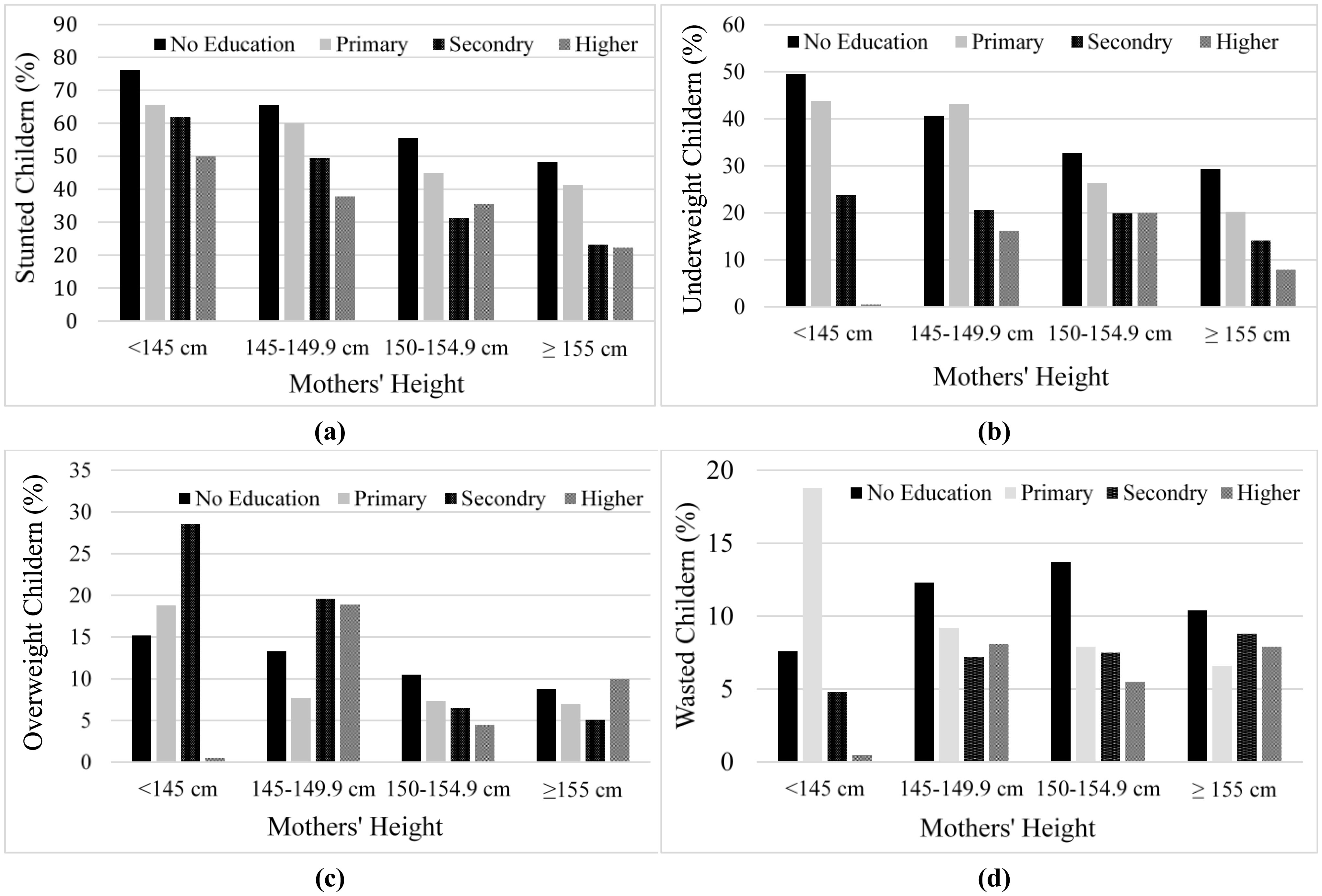
Pakistan has a significantly higher prevalence of stunted children under five years old compared with other countries with a similar income level. Given maternal education is a modifiable factor, we analyzed whether education has a larger marginal effect on improving children's growth for shorter stature mothers. Pakistan Demographic and Health Survey of 2012–13 was analyzed, with a total of 3,883 of children under five years of age (belonged to 2,327 mothers). The results showed that the overall prevalence of stunting, underweight, wasting, and overweight in our sample was 45%, 26.2%, 9.9%, and 9.5%, respectively. Short stature mothers have a higher number of malnourished children as compared to taller mothers. Compared to tall stature mothers, short stature mothers at all education levels have a higher number of stunted and underweight children. Maternal education has a significant positive effect on children's growth. However, we did not find significant differences in the marginal effect of maternal education among mothers with different statures. Policies providing specialized care to children born to short stature mothers are crucial, along with emphasizing mothers' education. Moreover, a poverty elevation program is necessary as a significant fraction of childhood malnutrition is attributed to the wealth index.
Citation: Nazli Javid, Christy Pu. Maternal stature, maternal education and child growth in Pakistan: a cross-sectional study[J]. AIMS Public Health, 2020, 7(2): 380-392. doi: 10.3934/publichealth.2020032
Pakistan has a significantly higher prevalence of stunted children under five years old compared with other countries with a similar income level. Given maternal education is a modifiable factor, we analyzed whether education has a larger marginal effect on improving children's growth for shorter stature mothers. Pakistan Demographic and Health Survey of 2012–13 was analyzed, with a total of 3,883 of children under five years of age (belonged to 2,327 mothers). The results showed that the overall prevalence of stunting, underweight, wasting, and overweight in our sample was 45%, 26.2%, 9.9%, and 9.5%, respectively. Short stature mothers have a higher number of malnourished children as compared to taller mothers. Compared to tall stature mothers, short stature mothers at all education levels have a higher number of stunted and underweight children. Maternal education has a significant positive effect on children's growth. However, we did not find significant differences in the marginal effect of maternal education among mothers with different statures. Policies providing specialized care to children born to short stature mothers are crucial, along with emphasizing mothers' education. Moreover, a poverty elevation program is necessary as a significant fraction of childhood malnutrition is attributed to the wealth index.

| [1] |
Black RE, Victora CG, Walker SP, et al. (2013) Maternal and child undernutrition and overweight in low-income and middle-income countries. Lancet 382: 427-451. doi: 10.1016/S0140-6736(13)60937-X

|
| [2] |
Adair LS, Fall CH, Osmond C, et al. (2013) Associations of linear growth and relative weight gain during early life with adult health and human capital in countries of low and middle income: findings from five birth cohort studies. Lancet 382: 525-534. doi: 10.1016/S0140-6736(13)60103-8
|
| [3] |
Hoddinott J, Alderman H, Behrman JR, et al. (2013) The economic rationale for investing in stunting reduction. Matern Child Nutr 69-82. doi: 10.1111/mcn.12080
|
| [4] | WHO (2019) Levels and trends in child malnutrition. Available from: https://www.who.int/nutgrowthdb/jme-2019-key-findings.pdf?ua=1. |
| [5] | UNICEF (2018) Four out of ten of the world's stunted children live in South Asia. Available from: http://www.unicefrosa-progressreport.org/stopstunting.html. |
| [6] |
Ozaltin E, Hill K, Subramanian SV, et al. (2010) Association of Maternal Stature With Offspring Mortality, Underweight, and Stunting in Low- to Middle-Income Countries. Jama 303: 1507-1516. doi: 10.1001/jama.2010.450
|
| [7] | WHO Multicentre Growth Reference Study Group (2006) WHO Child Growth Standards based on length/height, weight and age. Acta Paediatr 450: 76-85. |
| [8] |
Addo OY, Stein AD, Fall CH, et al. (2013) Maternal height and child growth patterns. J Pediatr 163: 549-554. doi: 10.1016/j.jpeds.2013.02.002
|
| [9] |
Hernandezdiaz S, Peterson KE, Dixit S, et al. (1999) Association of maternal short stature with stunting in Mexican children: common genes vs common environment. Eur J Clin Nutr 53: 938-945. doi: 10.1038/sj.ejcn.1600876
|
| [10] |
Sinha B, Taneja S, Chowdhury R, et al. (2018) Low-birthweight infants born to short-stature mothers are at additional risk of stunting and poor growth velocity: Evidence from secondary data analyses. Matern Child Nutr 14: e12504. doi: 10.1111/mcn.12504
|
| [11] |
Witter FR, Luke B (1991) The effect of maternal height on birth weight and birth length. Early Hum Dev 25: 181-186. doi: 10.1016/0378-3782(91)90114-I
|
| [12] |
Jananthan R, Wijesinghe D, Sivananthewerl T, et al. (2010) Maternal Anthropometry as a Predictor of Birth Weight. Trop Agric Res 21: 89-98. doi: 10.4038/tar.v21i1.2590
|
| [13] |
Hart N (1993) Famine, Maternal Nutrition and Infant Mortality: A Re-examination of the Dutch Hunger Winter. Pop Stud J Demog 47: 27-46. doi: 10.1080/0032472031000146716
|
| [14] |
Aoun N, Matsuda H, Sekiyama M, et al. (2015) Geographical accessibility to healthcare and malnutrition in Rwanda. Soc Sci Med 135-145. doi: 10.1016/j.socscimed.2015.02.004
|
| [15] |
Abuya BA, Onsomu EO, Kimani JK, et al. (2011) Influence of Maternal Education on Child Immunization and Stunting in Kenya. Matern Child Health J 15: 1389-1399. doi: 10.1007/s10995-010-0670-z
|
| [16] |
Makoka D, Masibo PK (2015) Is there a threshold level of maternal education sufficient to reduce child undernutrition? Evidence from Malawi, Tanzania and Zimbabwe. BMC Pediatr 15: 96-96. doi: 10.1186/s12887-015-0406-8
|
| [17] |
Bhutta ZA, Das JK, Rizvi A, et al. (2013) Evidence-based Interventions for Improvement of Maternal and Child Nutrition: What Can Be Done and at What Cost? Lancet 382: 452-477. doi: 10.1016/S0140-6736(13)60996-4
|
| [18] |
Limwattananon S, Tangcharoensathien V, Prakongsai P, et al. (2010) Equity in maternal and child health in Thailand. Bull World Health Organ 88: 420-427. doi: 10.2471/BLT.09.068791
|
| [19] | Pakistan (2013) Pakistan demographic and health survey 2012–13. NIPS and ICF International Islamabad, Pakistan, and Calverton, Maryland, USA . |
| [20] | Human-Rights-Watch, Barriers to Girls' Education in Pakistan. Available from: https://www.hrw.org/report/2018/11/12/shall-i-feed-my-daughter-or-educate-her/barriers-girls-education-pakistan. |
| [21] | Ali SB, Amir, Ashraf S, et al. (2018) Factors Associated with Stunting among Children Under Five Years of Age in Pakistan: Evidence from PDHS 2012–13. J Community Public Health Nurs 4: 1-4. |
| [22] |
Khan S, Zaheer S, Safdar NF, et al. (2019) Determinants of stunting, underweight and wasting among children < 5 years of age: evidence from 2012–2013 Pakistan demographic and health survey. BMC Public Health 19: 1-15. doi: 10.1186/s12889-018-6343-3
|
| [23] |
Rizvi A, Bhatti Z, Das JK, et al. (2015) Pakistan and the Millennium Development Goals for Maternal and Child Health: progress and the way forward. Paediatr Int Child Health 35: 287-297. doi: 10.1080/20469047.2015.1109257
|
| [24] | Barker DJP (1998) Mothers, babies, and health in later life Elsevier Health Sciences. |
| [25] |
Feng A, Wang L, Chen X, et al. (2015) Developmental Origins of Health and Disease (DOHaD): Implications for health and nutritional issues among rural children in China. Biosci Trends 9: 82-87. doi: 10.5582/bst.2015.01008
|
| [26] | The Demographic and Health Survey Program. Available from: https://dhsprogram.com/. |
| [27] | USAID-DHSAvailable from: https://www.usaid.gov/news-information/fact-sheets/demographic-health-survey. |
| [28] | Demographic and Health Survey Program Aims. Available from: https://dhsprogram.com/data/Guide-to-DHS-Statistics/Description_of_The_Demographic_and_Health_Surveys_Program.htm. |
| [29] |
Gage AJ (2007) Barriers to the Utilization of Maternal Health Care in Rural Mali. Soc Sci Med 65: 1666-1682. doi: 10.1016/j.socscimed.2007.06.001
|
| [30] | National Institute of Population Studies (NIPS) [Pakistan] and ICF International (2013) Pakistan demographic and health survey 2012–13. |
| [31] |
Mei ZG, Grummer-Strawn LM (2007) Standard deviation of anthropometric Z-scores as a data quality assessment tool using the 2006 WHO growth standards: a cross country analysis. Bull World Health Organ 85: 441-448. doi: 10.2471/BLT.06.034421
|
| [32] |
Der G, Everitt BS (2012) Applied medical statistics using SAS CRC Press. doi: 10.1201/b12738
|
| [33] |
Dewey KG, Begum K (2011) Long-term consequences of stunting in early life. Matern Child Nutr 5-18. doi: 10.1111/j.1740-8709.2011.00349.x
|
| [34] |
Rachmi CN, Agho KE, Li M, et al. (2016) Stunting coexisting with overweight in 20–49-year-old Indonesian children: prevalence, trends and associated risk factors from repeated cross-sectional surveys. Public Health Nutr 19: 2698-2707. doi: 10.1017/S1368980016000926
|
| [35] |
Kumar D, Goel N, Mittal PC, et al. (2006) Influence of Infant-feeding Practices on Nutritional Status of Under-five Children. Indian J Pediatr 73: 417-421. doi: 10.1007/BF02758565
|
| [36] |
Kandala N, Madungu TP, Emina JB, et al. (2011) Malnutrition among children under the age of five in the Democratic Republic of Congo (DRC): does geographic location matter? BMC Public Health 11: 261-261. doi: 10.1186/1471-2458-11-261
|
| [37] | Haque MN (2013) Assessment of nutritional status of underfive children and its determinants in Sri Lanka. Master thesis, Faculty of Bioscience Engineering, 1-86. |
| [38] | Wirth JP, Rohner F, Petry N, et al. (2017) Assessment of the WHO Stunting Framework using Ethiopia as a case study. Matern Child Nutr 13. |
| [39] |
Semali IA, Tengiakessy A, Mmbaga EJ, et al. (2015) Prevalence and determinants of stunting in under-five children in central Tanzania: remaining threats to achieving Millennium Development Goal 4. BMC Public Health 15: 1153-1153. doi: 10.1186/s12889-015-2507-6
|
| [40] |
Kennedy G, Nantel G, Brouwer ID, et al. (2006) Does living in an urban environment confer advantages for childhood nutritional status? Analysis of disparities in nutritional status by wealth and residence in Angola, Central African Republic and Senegal. Public Health Nutr 9: 187-193. doi: 10.1079/PHN2005835
|
| [41] |
Dekker LH, Moraplazas M, Marin C, et al. (2010) Stunting Associated with Poor Socioeconomic and Maternal Nutrition Status and Respiratory Morbidity in Colombian Schoolchildren. Food Nutr Bull 31: 242-250. doi: 10.1177/156482651003100207
|
| [42] | WHO (2016) Global strategy on diet, physical activity and health. Available from: https://www.who.int/dietphysicalactivity/childhood/en/. |
| [43] | Asian Development Bank (2015) Poverty Data: Pakistan. Available from: https://www.adb.org/countries/pakistan/poverty. 2015. |
Figures(1) / Tables(3)

Nazli Javid, Christy Pu. Maternal stature, maternal education and child growth in Pakistan: a cross-sectional study[J]. AIMS Public Health, 2020, 7(2): 380-392. doi: 10.3934/publichealth.2020032


 DownLoad: