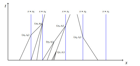
In this article, we focus on the BV regularity of the adapted entropy solutions of the conservation laws whose flux function contains infinitely many discontinuities with possible accumulation points. It is well known that due to discontinuities of the flux function in the space variable, the total variation of the solution can blow up to infinity in finite time. We establish the existence of total variation bounds for certain classes of fluxes and the initial data. Furthermore, we construct two counterexamples, which exhibit $ {\rm{BV}} $ blow-up of the entropy solution. These counterexamples not only demonstrate that these assumptions are essential, but also show that the BV-regularity result of [S. S. Ghoshal, J. Differential Equations, 258 (3), 980-1014, 2015] does not hold true when the spatial discontinuities of the flux are infinite.
Citation: Shyam Sundar Ghoshal, John D. Towers, Ganesh Vaidya. BV regularity of the adapted entropy solutions for conservation laws with infinitely many spatial discontinuities[J]. Networks and Heterogeneous Media, 2024, 19(1): 196-213. doi: 10.3934/nhm.2024009
In this article, we focus on the BV regularity of the adapted entropy solutions of the conservation laws whose flux function contains infinitely many discontinuities with possible accumulation points. It is well known that due to discontinuities of the flux function in the space variable, the total variation of the solution can blow up to infinity in finite time. We establish the existence of total variation bounds for certain classes of fluxes and the initial data. Furthermore, we construct two counterexamples, which exhibit $ {\rm{BV}} $ blow-up of the entropy solution. These counterexamples not only demonstrate that these assumptions are essential, but also show that the BV-regularity result of [S. S. Ghoshal, J. Differential Equations, 258 (3), 980-1014, 2015] does not hold true when the spatial discontinuities of the flux are infinite.

| [1] |
A. Adimurthi, S. S. Ghoshal, R. Dutta, G. D. Veerappa Gowda, Existence and nonexistence of TV bounds for scalar conservation laws with discontinuous flux, Comm. Pure Appl. Math., 64 (2011), 84–115. https://doi.org/10.1002/cpa.20346 doi: 10.1002/cpa.20346

|
| [2] |
A. Adimurthi, J. Jaffré, G. D. Veerappa Gowda, Godunov-type methods for conservation laws with a flux function discontinuous in space, SIAM J. Numer. Anal. 42 (2004), 179–208. https://doi.org/10.1137/S003614290139562X doi: 10.1137/S003614290139562X
|
| [3] |
A. Adimurthi, S. Mishra, G. D. Veerappa Gowda, Optimal entropy solutions for conservation laws with discontinuous flux functions, J. Hyperbolic Differ. Equ., 2 (2005), 783–837. https://doi.org/10.1142/S0219891605000622 doi: 10.1142/S0219891605000622
|
| [4] |
A. Adimurthi, S. Mishra, G. D. Veerappa Gowda, Convergence of Godunov type methods for a conservation law with a spatially varying discontinuous flux function. Math. Comp., 76 (2007), 1219–1242. https://doi.org/10.1090/S0025-5718-07-01960-6 doi: 10.1090/S0025-5718-07-01960-6
|
| [5] | A. Adimurthi, G. D. Veerappa Gowda, Conservation law with discontinuous flux, J. Math. Kyoto Univ., 43 (2003), 27–70. |
| [6] |
B. Andreianov, C. Cancés, Vanishing capillarity solutions of buckley–leverett equation with gravity in two-rocks medium, Comput. Geosci., 17 (2013), 551–572. https://doi.org/10.1007/s10596-012-9329-8 doi: 10.1007/s10596-012-9329-8
|
| [7] |
B. Andreianov, K. H. Karlsen, N. H. Risebro, A theory of $L^1$-dissipative solvers for scalar conservation laws with discontinuous flux, Arch. Ration. Mech. Anal., 201 (2011), 27–86. https://doi.org/10.1007/s00205-010-0389-4 doi: 10.1007/s00205-010-0389-4
|
| [8] |
E. Audusse, B. Perthame, Uniqueness for scalar conservation laws with discontinuous flux via adapted entropies, Proc. Roy. Soc. Edinburgh Sect. A, 135 (2005), 253–265. https://doi.org/10.1017/S0308210500003863 doi: 10.1017/S0308210500003863
|
| [9] |
R. Bürger, A. García, K. Karlsen, J. D. Towers, A family of numerical schemes for kinematic flows with discontinuous flux, J. Eng. Math., 60 (2008), 387–425. https://doi.org/10.1007/s10665-007-9148-4 doi: 10.1007/s10665-007-9148-4
|
| [10] |
R. Bürger, A. García, K. H. Karlsen, J. D. Towers, On an extended clarifier-thickener model with singular source and sink terms, European J. Appl. Math., 17 (2006), 257–292. https://doi.org/10.1017/S0956792506006619 doi: 10.1017/S0956792506006619
|
| [11] |
R. Bürger, K. H. Karlsen, N. H. Risebro, J. D. Towers, Well-posedness in $BV_t$ and convergence of a difference scheme for continuous sedimentation in ideal clarifier-thickener units, Numer. Math., 97 (2004), 25–65. https://doi.org/10.1007/s00211-003-0503-8 doi: 10.1007/s00211-003-0503-8
|
| [12] |
R. Bürger, K. H. Karlsen, J. D. Towers, An Engquist-Osher-type scheme for conservation laws with discontinuous flux adapted to flux connections, SIAM J. Numer. Anal. 47 (2009), 1684–1712. https://doi.org/10.1137/07069314X doi: 10.1137/07069314X
|
| [13] |
G. Q. Chen, N. Even, C. Klingenberg, Hyperbolic conservation laws with discontinuous fluxes and hydrodynamic limit for particle systems, J. Differ. Equ., 245 (2008), 3095–3126. https://doi.org/10.1016/j.jde.2008.07.036 doi: 10.1016/j.jde.2008.07.036
|
| [14] |
S. Diehl, A conservation law with point source and discontinuous flux function modelling continuous sedimentation, SIAM J. Appl. Math., 56 (1996), 388–419. https://doi.org/10.1137/S0036139994242425 doi: 10.1137/S0036139994242425
|
| [15] |
M. Garavello, R. Natalini, B. Piccoli, A. Terracina, Conservation laws with discontinuous flux, Netw. Heterog. Media., 2 (2007), 159–179. https://doi.org/10.3934/nhm.2007.2.159 doi: 10.3934/nhm.2007.2.159
|
| [16] | S. S. Ghoshal, Optimal results on TV bounds for scalar conservation laws with discontinuous flux, J. Differential Equations, 258 (2015), 3,980–1014. |
| [17] |
S. S. Ghoshal, BV regularity near the interface for nonuniform convex discontinuous flux, Netw. Heterog. Media., 11 (2016), 331–348. https://doi.org/10.3934/nhm.2016.11.331 doi: 10.3934/nhm.2016.11.331
|
| [18] |
S. S. Ghoshal, A. Jana, J. D. Towers, Convergence of a Godunov scheme to an Audusse-Perthame adapted entropy solution for conservation laws with BV spatial flux, Numer. Math., 146 (2020), 629–659. https://doi.org/10.1007/s00211-020-01150-y doi: 10.1007/s00211-020-01150-y
|
| [19] |
S. S. Ghoshal, S. Junca, A. Parmar, Fractional regularity for conservation laws with discontinuous flux, Nonlinear Anal. Real World Appl., 75 (2024), 103960. https://doi.org/10.1016/j.nonrwa.2023.103960 doi: 10.1016/j.nonrwa.2023.103960
|
| [20] |
S. S. Ghoshal, J. D. Towers, G. Vaidya, A Godunov type scheme and error estimates for scalar conservation laws with Panov-type discontinuous flux, Numer. Math., 151 (2022), 601–625. https://doi.org/10.1007/s00211-022-01297-w doi: 10.1007/s00211-022-01297-w
|
| [21] |
S. S. Ghoshal, J. D. Towers, G. Vaidya, Convergence of a Godunov scheme for conservation laws with degeneracy and BV spatial flux and a study of Panov type fluxes, J. Hyperbolic Differ. Equ., 19 (2022), 365–390. https://doi.org/10.1142/S0219891617500229 doi: 10.1142/S0219891617500229
|
| [22] | S. S. Ghoshal, J. D. Towers, and G. Vaidya. Well-posedness for conservation laws with spatial heterogeneities and a study of BV regularity, arXiv: 2010.13695 [Preprint], (2020), [cited 2024 Feb 18]. Available from: https://doi.org/10.48550/arXiv.2010.13695 |
| [23] |
K. H. Karlsen, J. D. Towers, Convergence of the Lax-Friedrichs scheme and stability for conservation laws with a discontinuous space-time dependent flux, Chinese Ann. Math. Ser. B, 25 (2004), 287–318. https://doi.org/10.1142/S0252959904000299 doi: 10.1142/S0252959904000299
|
| [24] |
K. H. Karlsen, J. D. Towers, Convergence of a Godunov scheme for conservation laws with a discontinuous flux lacking the crossing condition, J. Hyperbolic Differ. Equ., 14 (2017), 671–701. https://doi.org/10.1142/S0219891617500229 doi: 10.1142/S0219891617500229
|
| [25] |
S. Mishra, Convergence of upwind finite difference schemes for a scalar conservation law with indefinite discontinuities in the flux function, SIAM J. Numer. Anal., 43 (2005), 559–577. https://doi.org/10.1137/030602745 doi: 10.1137/030602745
|
| [26] |
S. N. Kružkov, First order quasilinear equations in several independent variables. Math. USSR Sb., 10 (1970), 217–243. https://doi.org/10.1070/SM1970v010n02ABEH002156 doi: 10.1070/SM1970v010n02ABEH002156
|
| [27] |
E. Y. Panov, On existence and uniqueness of entropy solutions to the Cauchy problem for a conservation law with discontinuous flux, J. Hyperbolic Differ. Equ., 6 (2009), 525–548. https://doi.org/10.1142/S0219891609001915 doi: 10.1142/S0219891609001915
|
| [28] |
B. Piccoli, M. Tournus, A general bv existence result for conservation laws with spatial heterogeneities, SIAM J. Math. Anal., 50 (2018), 2901–2927. https://doi.org/10.1137/17M112628X doi: 10.1137/17M112628X
|
| [29] |
W. Shen, On the uniqueness of vanishing viscosity solutions for riemann problems for polymer flooding, Nonlinear Differ. Equ. Appl., 24 (2017), 24–37. https://doi.org/10.1007/s00030-017-0461-y doi: 10.1007/s00030-017-0461-y
|
| [30] |
J. D. Towers, Convergence of a difference scheme for conservation laws with a discontinuous flux, SIAM J. Numer. Anal., 38 (2000), 681–698. https://doi.org/10.1137/S0036142999363668 doi: 10.1137/S0036142999363668
|
| [31] |
J. D. Towers, An existence result for conservation laws having BV spatial flux heterogeneities–without concavity, J. Differ. Equ., 269 (2020), 5754–5764. https://doi.org/10.1016/j.jde.2020.04.016 doi: 10.1016/j.jde.2020.04.016
|


Figures(3)
Shyam Sundar Ghoshal, John D. Towers, Ganesh Vaidya. BV regularity of the adapted entropy solutions for conservation laws with infinitely many spatial discontinuities[J]. Networks and Heterogeneous Media, 2024, 19(1): 196-213. doi: 10.3934/nhm.2024009


 DownLoad: