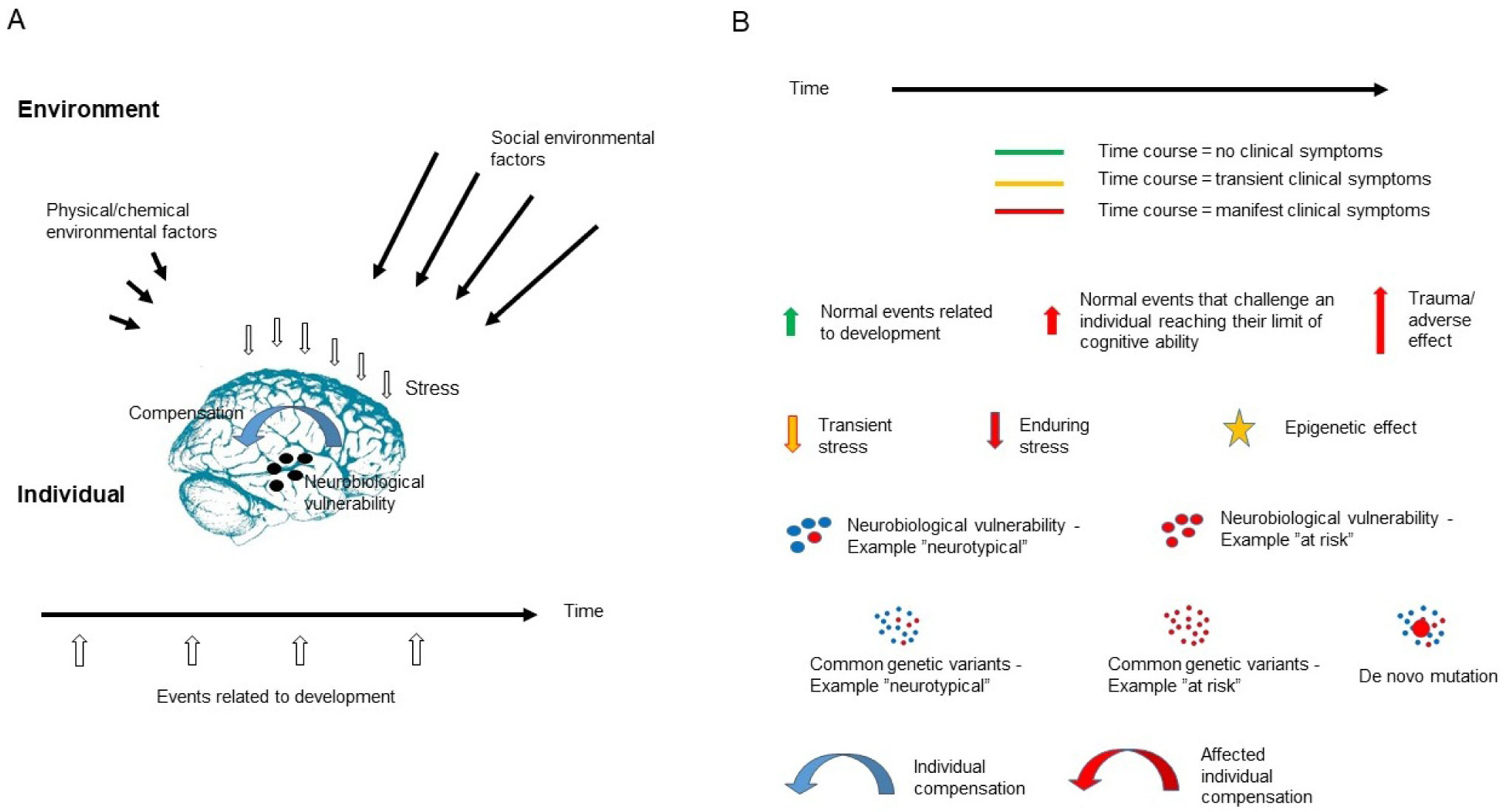
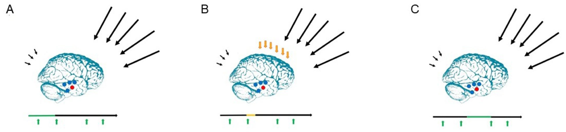
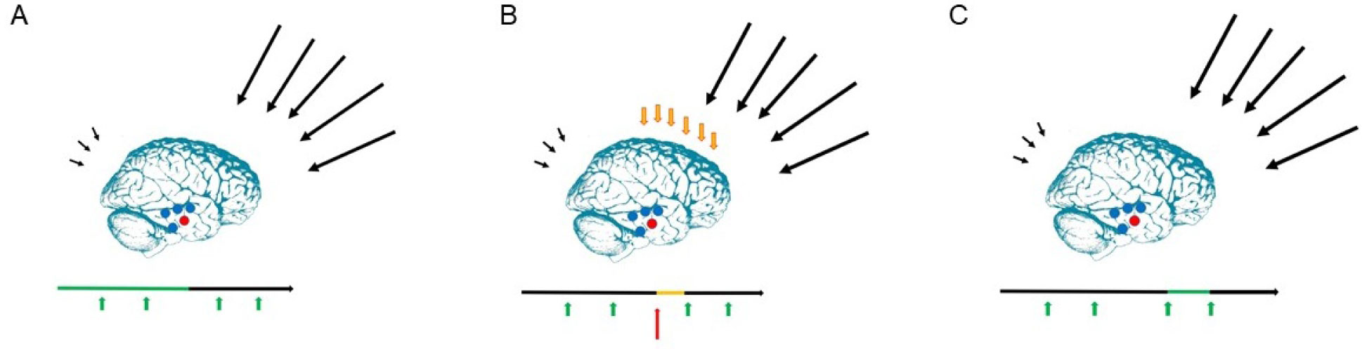
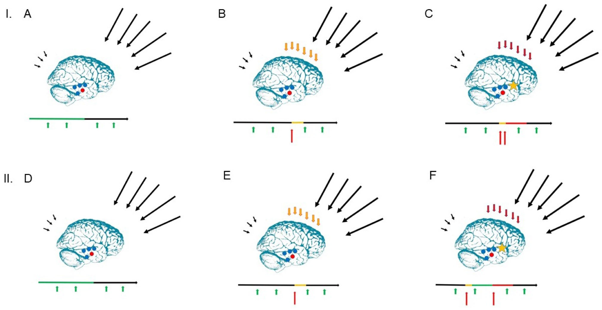
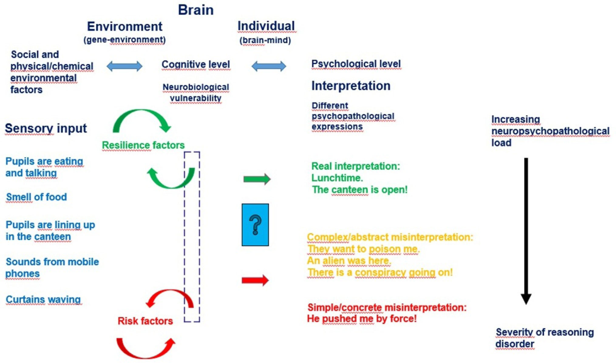
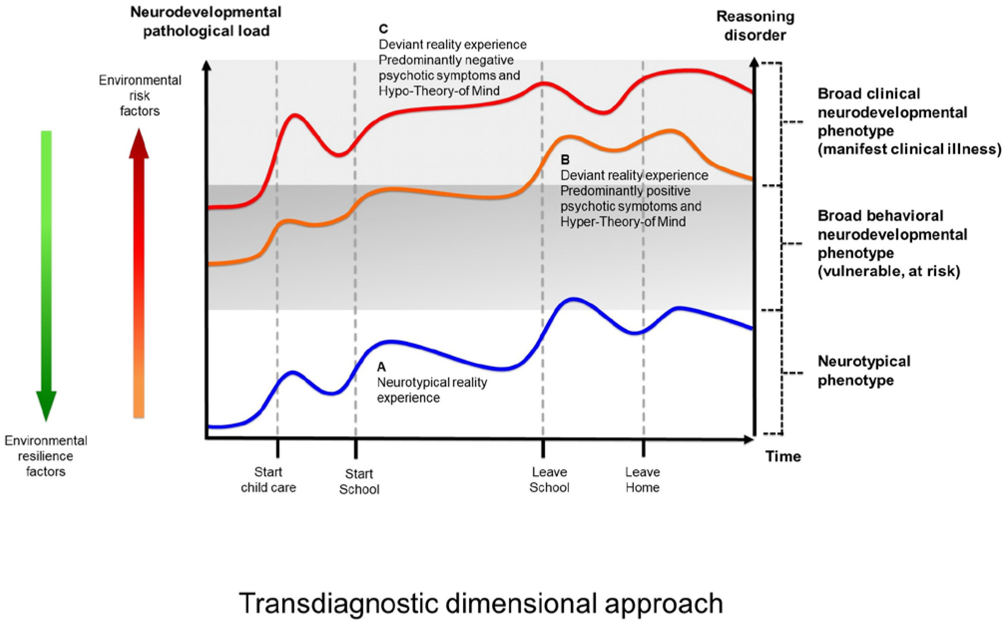
The present article is a theoretical contribution suggesting a simple model of the dynamics involved in the development of neurodevelopmental disorders and the phenomenon of autism offering an explanation of why different individuals have different onset of manifest disease. The model relates to present genetic and epigenetic evidence and previous theoretical models. The dynamic model applies an individualized transdiagnostic and dimensional approach integrating several levels of influence involved in the dynamic interaction between an individual and their environment across time. The dynamic model illustrates the interaction between a basic neurobiological susceptibility, compensating mechanisms, and stress-related releasing mechanisms involved in the development of manifest clinical illness. The model has a particular focus on the dynamics of neurocognitive processes and their relationship to more basic information, psychological and social processes. A basic assumption guiding the model is that even quite normal events related to typical development may increase the risk of enduring stress in cognitively vulnerable individuals, further increasing their risk of developing manifest clinical illness. The model suggests that genetic variation, endogenous epigenetic processes of development, and epigenetic changes influenced by physical/chemical and social environmental risk and resilience factors all may contribute to phenotypical expression. A genetic susceptibility may translate into a biological susceptibility reflected in cognitive impairments. A cognitively vulnerable individual may be at increased risk of misinterpreting sensory inputs, potentially resulting in psychopathological expressions, e.g., autistic symptoms, observed across several neurodevelopmental disorders. The genetically influenced experience of an individual relates to cognitive phenomena occurring at the interfaces between the brain, mind, and society. The severity of clinical illness may differ from the severity of a disorder of reasoning. The dynamic model may help guide future development of personalized medicine in psychiatry and identify relevant points of intervention. A discussion of the implications of the model relating to epigenetic evidence and to previous theoretical models is included at the end of the paper.
Citation: Bodil Aggernæs. Suggestion of a dynamic model of the development of neurodevelopmental disorders and the phenomenon of autism[J]. AIMS Molecular Science, 2020, 7(2): 122-182. doi: 10.3934/molsci.2020008
The present article is a theoretical contribution suggesting a simple model of the dynamics involved in the development of neurodevelopmental disorders and the phenomenon of autism offering an explanation of why different individuals have different onset of manifest disease. The model relates to present genetic and epigenetic evidence and previous theoretical models. The dynamic model applies an individualized transdiagnostic and dimensional approach integrating several levels of influence involved in the dynamic interaction between an individual and their environment across time. The dynamic model illustrates the interaction between a basic neurobiological susceptibility, compensating mechanisms, and stress-related releasing mechanisms involved in the development of manifest clinical illness. The model has a particular focus on the dynamics of neurocognitive processes and their relationship to more basic information, psychological and social processes. A basic assumption guiding the model is that even quite normal events related to typical development may increase the risk of enduring stress in cognitively vulnerable individuals, further increasing their risk of developing manifest clinical illness. The model suggests that genetic variation, endogenous epigenetic processes of development, and epigenetic changes influenced by physical/chemical and social environmental risk and resilience factors all may contribute to phenotypical expression. A genetic susceptibility may translate into a biological susceptibility reflected in cognitive impairments. A cognitively vulnerable individual may be at increased risk of misinterpreting sensory inputs, potentially resulting in psychopathological expressions, e.g., autistic symptoms, observed across several neurodevelopmental disorders. The genetically influenced experience of an individual relates to cognitive phenomena occurring at the interfaces between the brain, mind, and society. The severity of clinical illness may differ from the severity of a disorder of reasoning. The dynamic model may help guide future development of personalized medicine in psychiatry and identify relevant points of intervention. A discussion of the implications of the model relating to epigenetic evidence and to previous theoretical models is included at the end of the paper.

| [1] |
Baird G, Simonoff E, Pickles A, et al. (2006) Prevalence of disorders of the autism spectrum in a population cohort of children in South Thames: the Special Needs and Autism Project (SNAP). Lancet 368: 210-215. doi: 10.1016/S0140-6736(06)69041-7

|
| [2] |
Baxter AJ, Brugha TS, Erskine HE, et al. (2015) The epidemiology and global burden of autism spectrum disorders. Psychol Med 45: 601-613. doi: 10.1017/S003329171400172X
|
| [3] |
Brugha TS, Spiers N, Bankart J, et al. (2016) Epidemiology of autism in adults across age groups and ability levels. Br J Psychiatry 209: 498-503. doi: 10.1192/bjp.bp.115.174649
|
| [4] |
Elsabbagh M, Divan G, Koh Y-J, et al. (2012) Global prevalence of autism and other pervasive developmental disorders. Autism Res 5: 160-179. doi: 10.1002/aur.239
|
| [5] |
Atladottir HO, Gyllenberg D, Langridge A, et al. (2015) The increasing prevalence of reported diagnoses of childhood psychiatric disorders: a descriptive multinational comparison. Eur Child Adolesc Psychiatry 24: 173-183. doi: 10.1007/s00787-014-0553-8
|
| [6] |
Hansen SN, Schendel DE, Parner ET (2015) Explaining the increase in the prevalence of autism spectrum disorders. The proportion attributable to changes in reporting practices. JAMA Pediatr 169: 56-62. doi: 10.1001/jamapediatrics.2014.1893
|
| [7] |
Simonoff E (2012) Autism spectrum disorder: prevalence and cause may be bound together. Br J Psych 201: 88-89. doi: 10.1192/bjp.bp.111.104703
|
| [8] |
Gillberg C (2010) The ESSENCE in child psychiatry: Early Symptomatic Syndromes Eliciting Neurodevelopmental Clinical Examinations. Res Dev Dis 31: 1543-1551. doi: 10.1016/j.ridd.2010.06.002
|
| [9] |
Grove J, Ripke S, Als TD, et al. (2019) Identification of common genetic risk variants for autism spectrum disorder. Nat Genet 51: 431-444. doi: 10.1038/s41588-019-0344-8
|
| [10] |
Simonoff E, Pickles A, Charman, et al. (2008) Psychiatric disorders in children with autism spectrum disorders: Prevalence, comorbidity, and associated factors in a population-derived sample. J Am Acad Child Adolesc Psychiatry 47: 921-929. doi: 10.1097/CHI.0b013e318179964f
|
| [11] |
Wender CLA, Veenstra-VanderWeele J (2017) Challenge and Potential for Research on Gene-Environment Interactions in Autism Spectrum Disorder. Gene-Environment Transactions in Developmental Psychopathology, Advances in Development and Psychopathology: Brain Research Foundation Symposium Series 2 Springer International Publishing AG, 157-176. doi: 10.1007/978-3-319-49227-8_9
|
| [12] |
Sandin S, Lichtenstein P, Kuja-Halkola R, et al. (2014) The familial risk of autism. JAMA 311: 1770-1777. doi: 10.1001/jama.2014.4144
|
| [13] |
Robinson EB, St Pourcain B, Anttila V, et al. (2016) Genetic risk for autism spectrum disorders and neuropsychiatric variation in the general population. Nat Genet 48: 552-555. doi: 10.1038/ng.3529
|
| [14] |
Craddock N, Owen M (2010) The Kraepelinian dichotomy – going, going…but still not gone. Br J Psychiatry 196: 92-95. doi: 10.1192/bjp.bp.109.073429
|
| [15] | Cross-Disorder Group of the Psychiatric Genomics Consortium (2013) Identification of risk loci with shared effects on five major psychiatric disorders: a genome-wide analysis. Lancet 381: 1371-1379. |
| [16] |
Aggernæs B (2018) Autism: A transdiagnostic, dimensional construct of reasoning? Eur J Neurosci 47: 515-533. doi: 10.1111/ejn.13599
|
| [17] | Aggernæs B (2016) Rethinking the concept of psychosis and the link between autism and Schizophrenia. Scand J Child Adol Psychiat Psychol 4: 4-11. |
| [18] | Bleuler E (1911) Dementia Praecox oder Gruppe der Schizophrenien Leipzig: Deuticke. |
| [19] | Piaget J (1967) La psychologie de l'intelligence Paris: A. Colin. |
| [20] | Alberoni F (1984) Movement and Institution New York: Columbia University Press. |
| [21] |
Aggernæs A, Haugsted R (1976) Experienced reality in three to six year old children: A study of direct reality testing. J Child Psychol Psychiat 17: 323-335. doi: 10.1111/j.1469-7610.1976.tb00407.x
|
| [22] |
Aggernæs A, Paikin H, Vitger J (1981) Experienced reality in schizophrenia: How diffuse is the defect in reality testing? Indian J Psychol Med 4: 1-13. doi: 10.1177/0975156419810101
|
| [23] |
Clemmensen L, van Os J, Skovgaard AM, et al. (2014) Hyper-Theory-of-Mind in children with psychotic experiences. PLoS ONE 9: e113082. doi: 10.1371/journal.pone.0113082
|
| [24] |
Hallmayer J, Cleveland S, Torres A, et al. (2011) Genetic heritability and shared environmental factors among twin pairs with autism. Arch Gen Psychiatry 68: 1095-1102. doi: 10.1001/archgenpsychiatry.2011.76
|
| [25] |
Latham KE, Sapienza C, Engel N (2012) The epigenetic lorax: gene–environment interactions in human health. Epigenomics 4: 383-402. doi: 10.2217/epi.12.31
|
| [26] |
Miake K, Hirasawa T, Koide T, et al. (2012) Epigenetics in autism and other neurodevelopmental diseases. Adv Exp Med Biol 724: 91-98. doi: 10.1007/978-1-4614-0653-2_7
|
| [27] |
Shanen NC (2006) Epigenetics of autism spectrum disorders. Human Molecular Genetics 15: R138-R150. doi: 10.1093/hmg/ddl213
|
| [28] |
Siniscalco D, Cirillo A, Bradstreet JJ, et al. (2013) Epigenetic findings in autism: New perspectives for therapy. Int J Environ Res Public Health 10: 4261-4273. doi: 10.3390/ijerph10094261
|
| [29] |
Belmonte MK, Cook EH, Anderson GM, et al. (2004) Autism as a disorder of neural information processing: directions for research and targets for therapy. Mol Psychiatry 9: 646-663. doi: 10.1038/sj.mp.4001499
|
| [30] |
Courchesne E (2002) Abnormal early brain development in autism. Mol Psychiatry 7: S21-S23. doi: 10.1038/sj.mp.4001169
|
| [31] |
Menon V (2011) Large-scale brain networks and psychopathology: A unifying triple network model. Trends Cogn Sci 15: 483-506. doi: 10.1016/j.tics.2011.08.003
|
| [32] |
Szatmari P (2000) The classification of autism, Asperger's syndrome, and pervasive developmental disorder. Can J Psychiat 45: 731-738. doi: 10.1177/070674370004500806
|
| [33] |
Szyf M (2009) Epigenetics, DNA methylation, and chromatin modifying drugs. Annu Rev Pharmacol Toxicol 49: 243-263. doi: 10.1146/annurev-pharmtox-061008-103102
|
| [34] |
Plomin R (2011) Commentary: Why are children in the same family so different? Non-shared environment three decades later. Int J Epidemiol 40: 582-592. doi: 10.1093/ije/dyq144
|
| [35] |
Larsson HJ, Eaton WW, Madsen KM, et al. (2005) Risk factors for autism: perinatal factors, parental psychiatric history, and socioeconomic status. Am J Epidemiol 161: 916-925. doi: 10.1093/aje/kwi123
|
| [36] |
Lauritsen MB, Pedersen CB, Mortensen PB (2005) Effects of familial risk factors and place of birth on the risk of autism: a nationwide registerbased study. J Child Psychol Psyc 46: 963-971. doi: 10.1111/j.1469-7610.2004.00391.x
|
| [37] |
Gardener H, Spiegelman D, Buka SL (2009) Prenatal risk factors for autism: comprehensive meta-analysis. Br J Psychiatry 195: 7-14. doi: 10.1192/bjp.bp.108.051672
|
| [38] | Ramaswami G, Geschwind DH (2018) Chapter 21 Genetics of autism spectrum disorder. Handbook of Clinical Neurology, Vol. 147 (3rd series) Neurogenetics, Part I Elsevier, 321-329. |
| [39] |
Betancur C (2011) Etiological heterogeneity in autism spectrum disorders: More than 100 genetic and genomic disorders and still counting. Brain Res 1380: 42-77. doi: 10.1016/j.brainres.2010.11.078
|
| [40] |
Nava C, Keren B, Mignot C, et al. (2014) Prospective diagnostic analysis of copy number variants using SNP microarrays in individuals with autism spectrum disorders. Eur J Hum Genet 22: 71-78. doi: 10.1038/ejhg.2013.88
|
| [41] | The Autism Genome Project Consortium (2007) Mapping autism risk loci using genetic linkage and chromosomal rearrangements. Nat Genet 39: 319-328. |
| [42] |
Weiner DJ, Wigdor EM, Ripke S, et al. (2017) Polygenic transmission disequilibrium confirms that common and rare variation act additively to create risk for autism spectrum disorders. Nat Genet 49: 978-985. doi: 10.1038/ng.3863
|
| [43] |
Gaugler T, Klei L, Sanders SJ, et al. (2014) Most genetic risk for autism resides with common variation. Nat Genet 46: 881-885. doi: 10.1038/ng.3039
|
| [44] |
Guilmatre A, Dubourg C, Mosca AL, et al. (2009) Recurrent rearrangements in synaptic and neurodevelopmental genes and shared biologic pathways in schizophrenia, autism, and mental retardation. Arch Gen Psychiat 66: 947-956. doi: 10.1001/archgenpsychiatry.2009.80
|
| [45] |
McCarthy SE, Gillis J, Kramer M, et al. (2014) De novo mutations in schizophrenia implicate chromatin remodeling and support a genetic overlap with autism and intellectual disability. Mol Psychiatry 19: 652-658. doi: 10.1038/mp.2014.29
|
| [46] |
Hannon E, Schendel D, Ladd-Acosta C, et al. (2018) Elevated polygenic burden for autism is associated with differential DNA methylation at birth. Genome Med 10: 19. doi: 10.1186/s13073-018-0527-4
|
| [47] | Tran NQV, Miyake K (2017) Neurodevelopmental disorders and environmental toxicants: epigenetics as an underlying mechanism. Int J Genomics 2017: 7526592. |
| [48] |
Waddington CH (2012) The epigenotype. Int J Epidemiol 41: 10-13. doi: 10.1093/ije/dyr184
|
| [49] |
Fraga MF, Ballestar E, Paz MF, et al. (2005) Epigenetic differences arise during the lifetime of monozygotic twins. Proc Natl Acad Sci USA 102: 10604-10609. doi: 10.1073/pnas.0500398102
|
| [50] |
Lee R, Avramopoulos D (2014) Introduction to Epigenetics in Psychiatry. Epigenetics in Psychiatry Elsevier Inc., 3-25. doi: 10.1016/B978-0-12-417114-5.00001-2
|
| [51] |
Bale TL (2014) Lifetime stress experience: transgenerational epigenetics and germ cell programming. Dialogues Clin Neurosci 16: 297-305. doi: 10.31887/DCNS.2014.16.3/tbale
|
| [52] | Gos M (2013) Epigenetic mechanisms of gene expression regulation in neurological diseases. Acta Neurobiol Exp 73: 19-37. |
| [53] |
James SJ, Melnyk S, Jernigan S, et al. (2006) Metabolic endophenotype and related genotypes are associated with oxidative stress in children with autism. Am J Med Genet Part B 141B: 947-956. doi: 10.1002/ajmg.b.30366
|
| [54] |
Deth R, Muratore C, Benzecry J, et al. (2008) How environmental and genetic factors combine to cause autism: A redox/methylation hypothesis. Neurotoxicology 29: 190-201. doi: 10.1016/j.neuro.2007.09.010
|
| [55] |
Homs A, Codina-Solà M, Rodríguez-Santiago B, et al. (2016) Genetic and epigenetic methylation defects and implication of the ERMN gene in autism spectrum disorders. Transl Psychiatry 6: e855. doi: 10.1038/tp.2016.120
|
| [56] |
Ginsberg MR, Rubin RA, Falcone T, et al. (2012) Brain transcriptional and epigenetic associations with autism. PLoS ONE 7: e44736. doi: 10.1371/journal.pone.0044736
|
| [57] |
Wong CCY, Meaburn EL, Ronald A, et al. (2014) Methylomic analysis of monozygotic twins discordant for autism spectrum disorder and related behavioural traits. Mol Psychiatry 19: 495-503. doi: 10.1038/mp.2013.41
|
| [58] |
Minnis H (2013) Maltreatment-Associated Psychiatric Problems: An Example of Environmentally Triggered ESSENCE? Sci World J 2013: 148468. doi: 10.1155/2013/148468
|
| [59] | Pritchett R, Pritchett J, Marshall E, et al. (2013) Reactive attachment disorder in the general population: a hidden ESSENCE disorder. Sci World J 2013: 81815. |
| [60] |
Dinkler L, Lundström S, Gajwani R, et al. (2017) Maltreatment-associated neurodevelopmental disorders: a co-twin control analysis. J Child Psychol Psychiatr 58: 691-701. doi: 10.1111/jcpp.12682
|
| [61] |
McEwen BS (2008) Central effects of stress hormones in health and disease: understanding the protective and damaging effects of stress and stress mediators. Eur J Pharmacol 583: 174-185. doi: 10.1016/j.ejphar.2007.11.071
|
| [62] | Rostène W, Sarrieau A, Nicot A, et al. (1995) Steroid effects on brain functions: An example of the action of glucocorticoids on central dopaminergic and neurotensinergic systems. J Psychiatry Neurosci 20: 349-356. |
| [63] |
Meaney MJ, Szyf M (2005) Environmental programming of stress responses through DNA methylation: life at the interface between a dynamic environment and a fixed genome. Dialogues Clin Neurosci 7: 103-123. doi: 10.31887/DCNS.2005.7.2/mmeaney
|
| [64] |
Weaver ICG, Champagne FA, Brown SE, et al. (2005) Reversal of maternal programming of stress responses in adult offspring through methyl supplementation: Altering epigenetic marking later in life. J Neurosci 25: 11045-11054. doi: 10.1523/JNEUROSCI.3652-05.2005
|
| [65] |
McGowan PO, Matthews SG (2018) Prenatal stress, glucocorticoids, and developmental programming of the stress response. Endocrinology 159: 69-82. doi: 10.1210/en.2017-00896
|
| [66] |
Stenz L, Schechter DS, Serpa SR, et al. (2018) Intergenerational transmission of DNA methylation signatures associated with early life stress. Curr Genomics 19: 665-675. doi: 10.2174/1389202919666171229145656
|
| [67] |
Oberlander TF, Weinberg J, Papsdorf M, et al. (2008) Prenatal exposure to maternal depression, neonatal methylation of human glucocorticoid receptor gene (NR3C1) and infant cortisol stress responses. Epigenetics 3: 97-106. doi: 10.4161/epi.3.2.6034
|
| [68] | Corbett BA, Mendoza S, Wegelin JA, et al. (2008) Variable cortisol circadian rhythms in children with autism and anticipatory stress. J Psychiatry Neurosci 33: 227-234. |
| [69] |
Corbett BA, Schupp CW, Levine S, et al. (2009) Comparing cortisol, stress, and sensory sensitivity in children with autism. Autism Res 2: 39-49. doi: 10.1002/aur.64
|
| [70] |
Corbett BA, Schupp CW, Lanni KE (2012) Comparing biobehavioral profiles across two social stress paradigms in children with and without autism spectrum disorders. Mol Autism 3: 13. doi: 10.1186/2040-2392-3-13
|
| [71] |
Corbett BA, Muscatello RA, Blain SD (2016) Impact of sensory sensitivity on physiological stress response and novel peer interaction in children with and without autism spectrum disorder. Front Neurosci 10: 278. doi: 10.3389/fnins.2016.00278
|
| [72] |
Tordjman S, Anderson GM, Kermarrec S, et al. (2014) Altered circadian patterns of salivary cortisol in low-functioning children and adolescents with autism. Psychoneuroendocrinology 50: 227-245. doi: 10.1016/j.psyneuen.2014.08.010
|
| [73] |
Bishop-Fitzpatrick L, Mazefsky CA, Minshew NJ, et al. (2015) The relationship between stress and social functioning in adults with autism spectrum disorder and without intellectual disability. Autism Res 8: 164-173. doi: 10.1002/aur.1433
|
| [74] |
Bishop-Fitzpatrick L, Minshew NJ, Mazefsky CA, et al. (2017) Perception of life as stressful, not biological response to stress, is associated with greater social disability in adults with autism spectrum disorder. Autism Dev Disord 47: 1-16. doi: 10.1007/s10803-016-2910-6
|
| [75] |
Sønderby IE, Gústafsson Ó, Doan NT, et al. (2018) Dose response of the 16p11.2 distal copy number variant on intracranial volume and basal ganglia. Mol Psychiatry 25: 584-602. doi: 10.1038/s41380-018-0118-1
|
| [76] |
Turner TN, Coe BP, Dickel DE, et al. (2017) Genomic patterns of de novo mutation in simplex autism. Cell 171: 710-722. doi: 10.1016/j.cell.2017.08.047
|
| [77] |
Schork AJ, Won H, Appadurai V, et al. (2019) A genome-wide association study of shared risk across psychiatric disorders implicates gene regulation during fetal neurodevelopment. Nat Neurosci 22: 353-361. doi: 10.1038/s41593-018-0320-0
|
| [78] |
Gandal MJ, Haney JR, Parikshak NN, et al. (2018) Shared molecular neuropathology across major psychiatric disorders parallels polygenic overlap. Science 359: 693-697. doi: 10.1126/science.aad6469
|
| [79] |
Shulha HP, Cheung I, Guo Y, et al. (2013) Coordinated cell type–specific epigenetic remodeling in prefrontal cortex begins before birth and continues into early adulthood. PLoS Genet 9: e1003433. doi: 10.1371/journal.pgen.1003433
|
| [80] |
Belmonte MK, Yurgelun-Todd DA (2003) Functional anatomy of impaired selective attention and compensatory processing in autism. Brain Res Cogn Res 17: 651-664. doi: 10.1016/S0926-6410(03)00189-7
|
| [81] |
Livingston LA, Happé F (2017) Conceptualising compensation in neurodevelopmental disorders: Reflections from autism spectrum disorders. Neurosci Biobehav Rev 80: 729-742. doi: 10.1016/j.neubiorev.2017.06.005
|
| [82] |
Weems CF (2015) Biological correlates of child and adolescent responses to disaster exposure: A bio-ecological model. Curr Psychiatry Rep 17: 1-7. doi: 10.1007/s11920-015-0588-7
|
| [83] |
Weems CF, Russel JD, Neill EL, et al. (2019) Annual Research Review: Pediatric posttraumatic stress disorder from a neurodevelopmental network perspective. J Child Psychol Psychiatr 60: 395-408. doi: 10.1111/jcpp.12996
|
| [84] | Ouss-Ryngaert L, Golse B (2010) Linking neuroscience and psychoanalysis from a developmental perspective: Why and how? J Physiol 104: 303-308. |
| [85] |
Hosman CMH, van Doesum KTM, van Santvoort F (2009) Prevention of emotional problems and psychiatric risks in children of parents with a mental illness in the Netherlands: I. The scientific basis to a comprehensive approach. Aust e-J Advancement Ment Health 8: 250-263. doi: 10.5172/jamh.8.3.250
|
| [86] | Sarovic D (2018) A framework for neurodevelopmental disorders: Operationalization of a pathogenetic triad for clinical and research use. Gillberg Neuropsychiatry Centre, Institute of Neuroscience and Physiology, Sahlgrenska Academy University of Gothenburg Available from: https://psyarxiv.com/mbeqh/. |
| [87] |
Caspi A, Houts RM, Belsky DW, et al. (2014) The p factor: One general psychopathology factor in the structure of psychiatric disorders? Clin Psychol Sci 2: 119-137. doi: 10.1177/2167702613497473
|
| [88] |
Sameroff AJ, Mackenzie MJ (2003) Research strategies for capturing transactional models of development: The limits of the possible. Dev Psychopathol 15: 613-640. doi: 10.1017/S0954579403000312
|
| [89] |
Bishop-Fitzpatrick L, Mazefsky CA, Eack SM (2018) The combined impact of social support and perceived stress on quality of life in adults with autism spectrum disorder and without intellectual disability. Autism 22: 703-711. doi: 10.1177/1362361317703090
|
| [90] |
Bishop-Fitzpatrick L, Smith LE, Greenberg JS, et al. (2017) Participation in recreational activities buffers the impact of perceived stress on quality of life in adults with autism spectrum disorder. Autism Res 10: 973-982. doi: 10.1002/aur.1753
|
| [91] |
Yehuda R, Lehrner A, Bierer LM (2018) The public reception of putative epigenetic mechanisms in the transgenerational effects of trauma. Environ Epigenet 4: 1-7. doi: 10.1093/eep/dvy018
|
| [92] |
Clarke T-K, Lupton MK, Fernandez-Pujals AM, et al. (2016) Common polygenic risk for autism spectrum disorder (ASD) is associated with cognitive ability in the general population. Mol Psychiatry 21: 419-425. doi: 10.1038/mp.2015.12
|
| [93] |
Robinson EB, Samocha KE, Kosmicki JA, et al. (2014) Autism spectrum disorder severity reflects the average contribution of de novo and familial influences. Proc Natl Acad Sci USA 111: 15161-15165. doi: 10.1073/pnas.1409204111
|
| [94] |
Sanders SJ, He X, Willsey AJ, et al. (2015) Insights into autism spectrum disorder genomic architecture and biology from 71 risk loci. Neuron 87: 1215-1233. doi: 10.1016/j.neuron.2015.09.016
|
| [95] |
Bakermans-Kranenburg MJ, van Ijzendoorn MH (2006) Gene-environment interaction of the dopamine D4 receptor (DRD4) and observed maternal insensitivity predicting externalizing behavior in preschoolers. Dev Psychobiol 48: 406-409. doi: 10.1002/dev.20152
|
| [96] |
Kumsta R, Stevens S, Brookes K, et al. (2010) 5HTT genotype moderates the influence of early institutional deprivation on emotional problems in adolescence: evidence from the English and Romanian Adoptee (ERA) study. J Child Psychol Psychiatry 51: 755-762. doi: 10.1111/j.1469-7610.2010.02249.x
|
| [97] |
Yang C-J, Tan H-P, Yang F-Y (2015) The cortisol, serotonin and oxytocin are associated with repetitive behavior in autism spectrum disorder. Res Autism Spectr Disord 18: 12-20. doi: 10.1016/j.rasd.2015.07.002
|
| [98] |
Meier SM, Petersen L, Schendel DE, et al. (2015) Obsessive-compulsive disorder and autism spectrum disorders: Longitudinal and offspring risk. PLoS ONE 10: e0141703. doi: 10.1371/journal.pone.0141703
|
| [99] |
Valla JM, Belmonte MK (2013) Detail-oriented cognitive style and social communicative deficits, within and beyond the autism spectrum: independent traits that grow into developmental interdependence. Dev Rev 33: 371-398. doi: 10.1016/j.dr.2013.08.004
|
| [100] |
Lai MC, Lombardo MV, Ruigrok AN, et al. (2017) Quantifying and exploring camouflaging in men and women with autism. Autism 21: 690-702. doi: 10.1177/1362361316671012
|
| [101] |
Atladóttir HO, Thorsen P, Schendel DE, et al. (2010) Association of hospitalization for infection in childhood with diagnosis of autism spectrum disorders. Arch Pediatr Adolesc Med 164: 470-477. doi: 10.1001/archpediatrics.2010.9
|
| [102] |
Nudel R, Wang Y, Appadurai V, et al. (2019) A large-scale genomic investigation of susceptibility to infection and its association with mental disorders in the Danish population. Transl Psychiatry 9: 283. doi: 10.1038/s41398-019-0622-3
|
| [103] |
Danese A, Moffitt TE, Arseneault L, et al. (2017) The origins of cognitive deficits in victimized children: Implications for neuroscientists and clinicians. Am J Psychiatry 174: 349-361. doi: 10.1176/appi.ajp.2016.16030333
|
| [104] |
Kim SY, Bottema-Beutel K (2019) A meta regression analysis of quality of life correlates in adults with ASD. Res Autism Spectr Disord 63: 23-33. doi: 10.1016/j.rasd.2018.11.004
|
| [105] |
Plana-Ripoll O, Pedersen CB, Holtz Y, et al. (2019) Exploring comorbidity within mental disorders among a danish national population. JAMA Psychiatry 76: 259-270. doi: 10.1001/jamapsychiatry.2018.3658
|
| [106] |
Cuthbert N, Insel R (2013) Toward the future of psychiatric diagnosis: the seven pillars of RDoC. BMC Med 11: 126. doi: 10.1186/1741-7015-11-126
|
| [107] | (2013) American Psychiatric AssociationDiagnostic and Statistical Manual of Mental Disorders. American Psychiatric Publishing. |
| [108] | (1993) WHOThe ICD-10 Classification of Mental and Behavioural Disorders: Diagnostic Criteria for Research. Geneva: World Health Organization. |
| [109] |
Polanczyk GV, Casella C, Jaffee SR (2019) Commentary: ADHD lifetime trajectories and the relevance of the developmental perspective to Psychiatry: reflections on Asherson and Agnew-Blais. J Child Psychol Psychiatry 60: 353-355. doi: 10.1111/jcpp.13050
|
| [110] |
Narusyte J, Neiderhiser JM, D'Onofrio BM, et al. (2008) Testing different types of genotype–environment correlation: An extended children-of-twins model. Dev Psychol 44: 1591-1603. doi: 10.1037/a0013911
|
| [111] |
Sykes NH, Lamb JA (2007) Autism: The quest for the genes. Expert Rev Mol Med 9: 1-15. doi: 10.1017/S1462399407000452
|
Figures(10) / Tables(2)

Bodil Aggernæs. Suggestion of a dynamic model of the development of neurodevelopmental disorders and the phenomenon of autism[J]. AIMS Molecular Science, 2020, 7(2): 122-182. doi: 10.3934/molsci.2020008


 DownLoad: