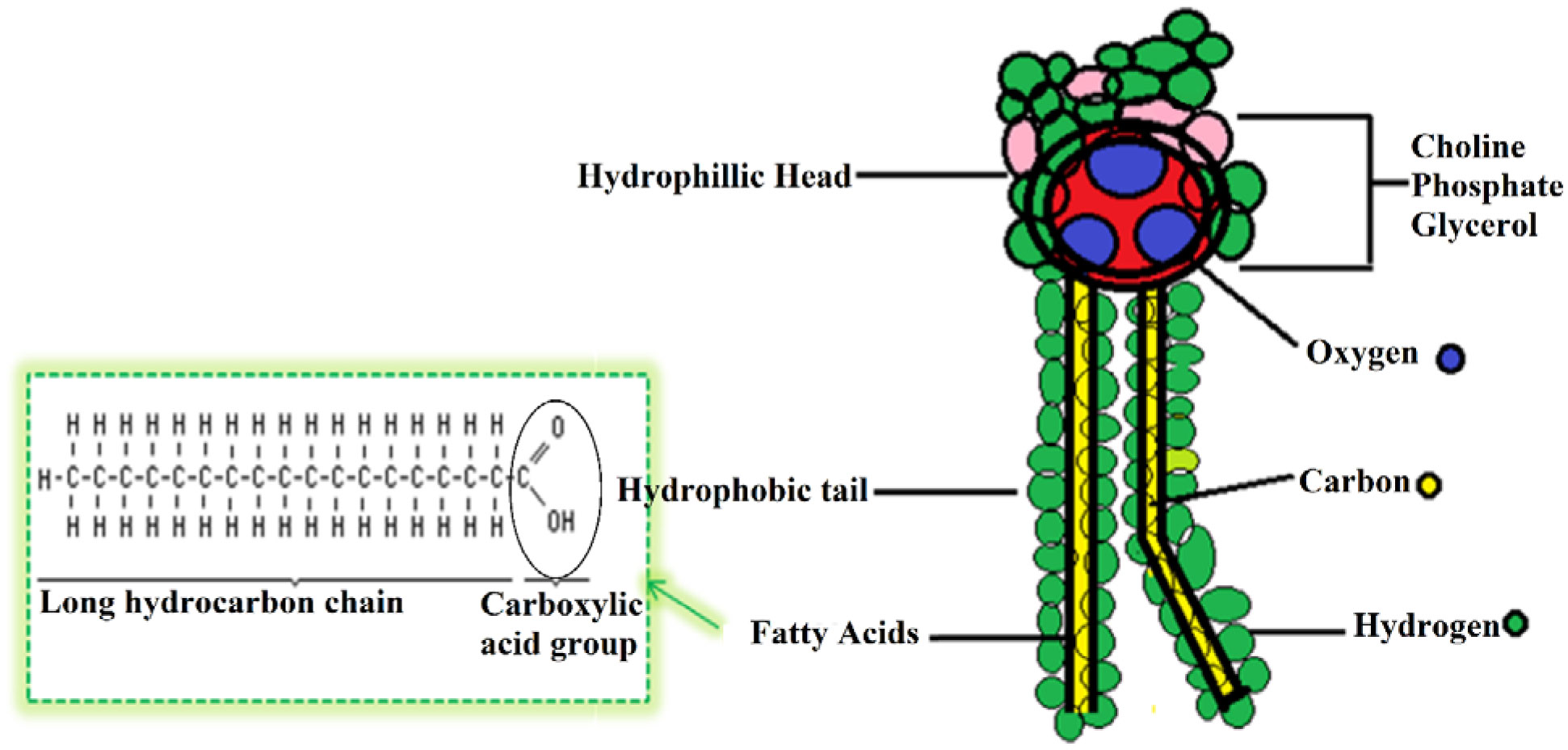
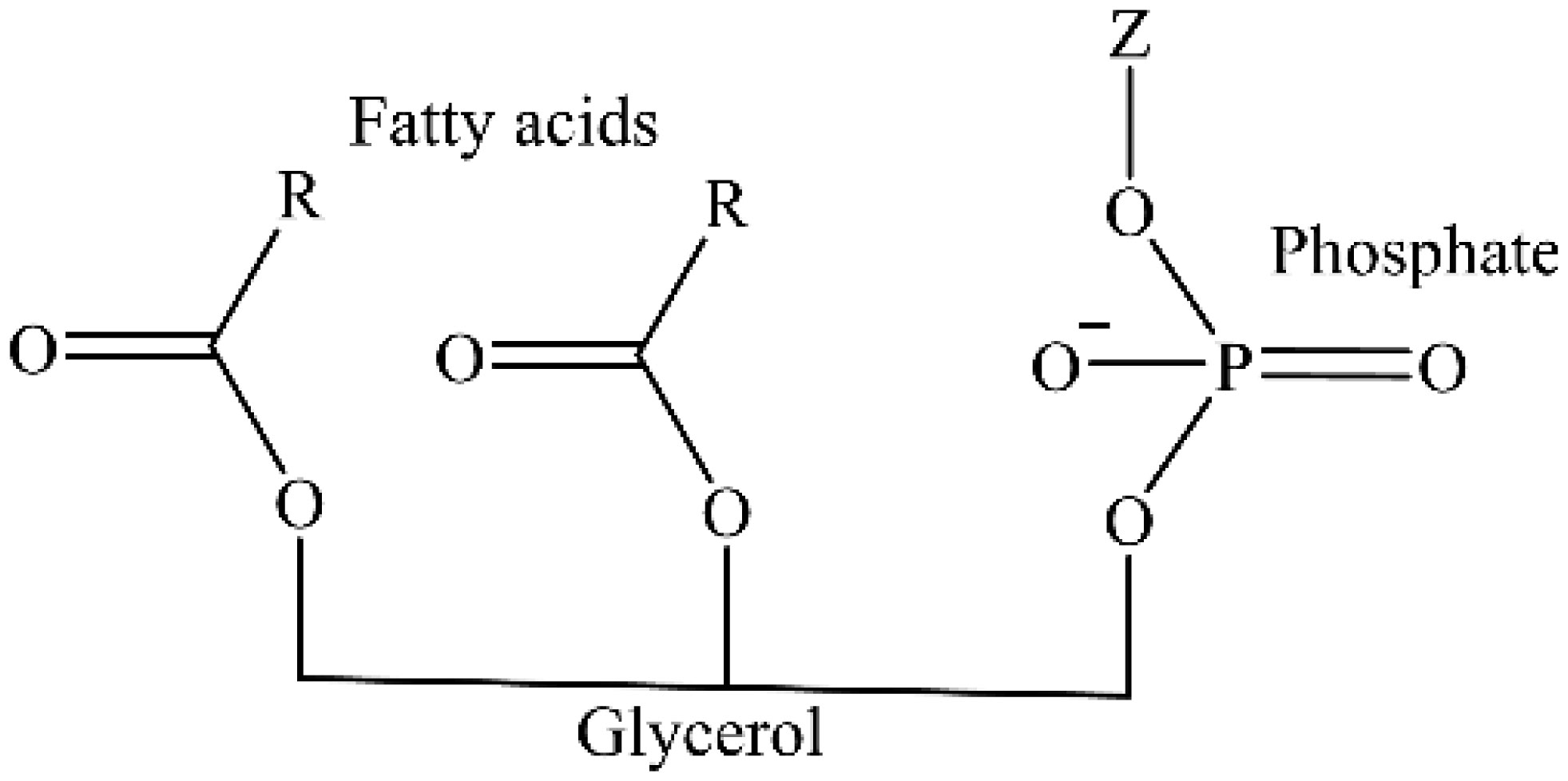
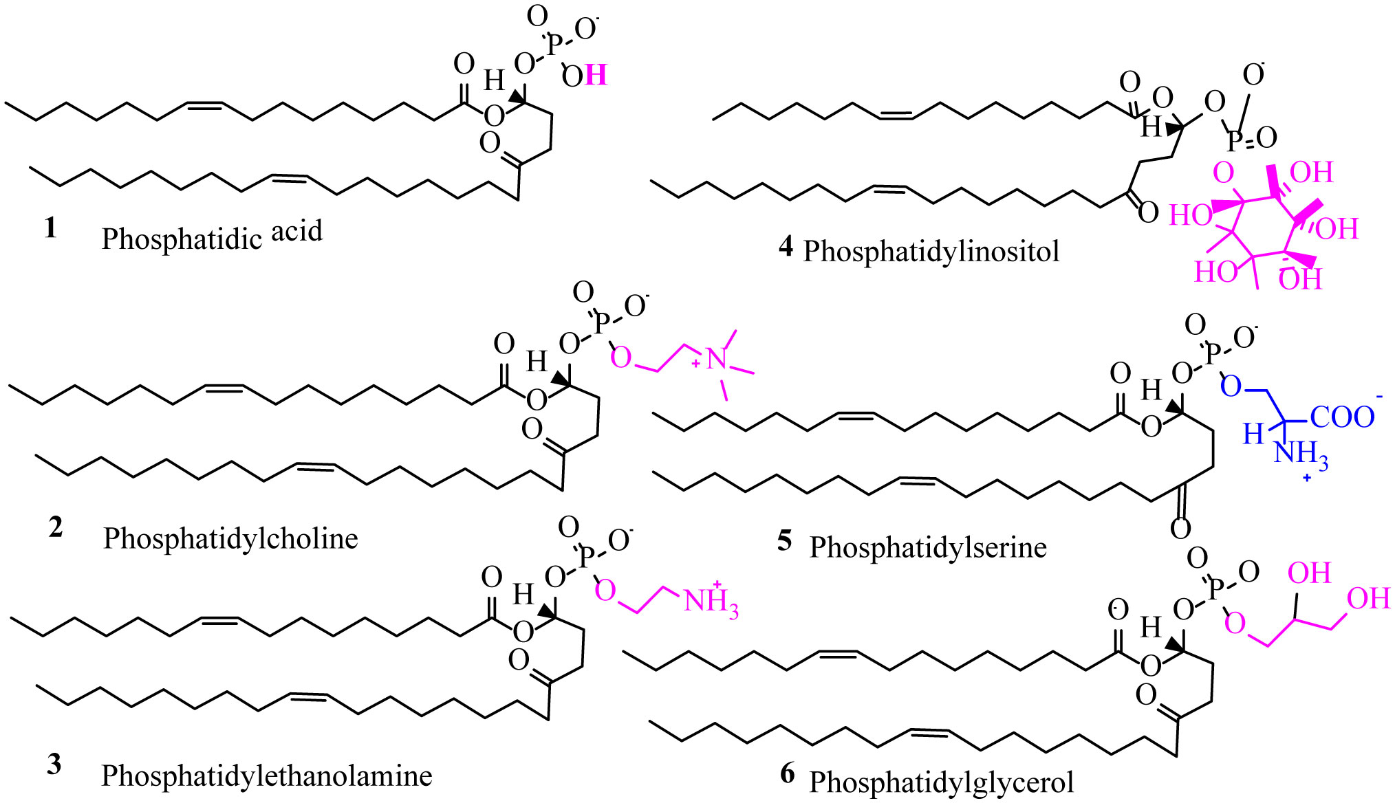
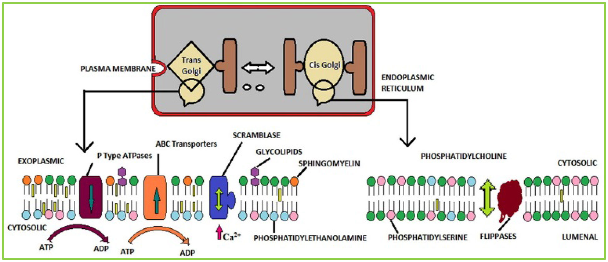
Phospholipids (PLs) are amphiphilic molecules that are in charge of controlling what goes in or out of the cell, keeping up the structure and numerous associated functions. These primary molecules are not only the integral part but also a vastly diverse group of molecules present in microorganisms, plants, and animals. PLs provide rigidity, signal transduction, energy to cells. PLs such as lecithins are molecules of future food, medicine and cosmetic industry. PLs are used in fat and oil refining and these are also used as carriers in drug and drug delivery system. Of course, challenges are there in the assay of phospholipids because of their availability of hydrophobic and hydrophilic components in the same environment. This review is mainly focused to unveil the function, characteristics, features and applications of PLs in various fields.
1.
Introduction
Reconstructing the stress and deformation history of a sedimentary basin is a challenging and important problem in the geosciences [32]. The mechanical response of a sedimentary basin is the consequence of complex multi-physics processes involving mechanical, geochemical, thermal and hydrological aspects. Among these, the inclusion of erosion or deposition of material plays a key role in the reconstruction of a sedimentary basin history.
A sedimentary basin is usually represented by a porous medium filled with water. To model surface erosion or deposition, we let the top surface of the basin evolve according to a given profile. The dynamics of erosion/deposition is affected by many complex phenomena, which are only partially accounted for in this study. Since the scope of this work is more focused on the methodology, precisely the development of a numerical solver, we address a simplified problem configuration which features a slab of porous, deformable material that is homogeneous, completely saturated with water and affected by a prescribed mixed erosion deposition profile on the top surface. In this way, we combine in a sigle model the mechanical, hydrological and erosion/deposition effects.
In this work we tackle the evolution of the top surface using the cut finite element method (CutFEM). This method is combined with a fixed-stress approach for solving the coupled flow and mechanics models. To deal with a moving boundary, the physical domain, is embedded in a larger computational grid. The evolution of top surface of the slab is described by the zero value of a time dependent level set function. The CutFEM approximation allows to handle the evolution of the top layer of the slab avoiding re-meshing techniques. However, depending on the intersection between the computational grid and the level set function, it can worsen the condition number of the problem. To overcome the ill-conditioning due to the CutFEM approximation, we propose the use of a stabilization terms and of a preconditioner applied to the fixed-stress splitting scheme.
On the basis of seminal works using the finite element method for the approximation of elliptic problems featuring unfitted boundaries and interfaces [9,15,20,21], the CutFEM method was developed and formalized as a general framework for simultaneously discretizing the geometry of the domain and the related partial differential equations [8]. Despite its many advantages, it is well known that this approach significantly worsens the conditioning of the discretized operators, because the finite element discretization is set on cut elements that may become arbitrarily small and skewed, according to the configuration of the unfitted boundary or interface with respect to the computational mesh. To override this issue, several techniques have been proposed. Stabilization techniques acting on the problem formulation have been successfully applied to this purpose [7,9,10,25,29]. It has been also shown that the ill-conditioning of the CutFEM discretization can be addressed by means of suitable preconditioners, [24,28,34]. Such techniques make CutFEM become a stable, efficient and robust method for a wide variety of problems, including second order elliptic equations [11,15,20], incompressible flow problems such as Stokes [19,22,25,28] and Navier-Stokes [29] and linear elasticity models [21]. However, the application of CutFEM to multi-physics problems involving the coupled CutFEM approximation of multiple variables is still rather unexplored. The scope of the present study is to shed light on some of the difficulties that appear in this context and to show how the available theory of CutFEM can be used to overcome these issues. In particular, we address a poromechanics problem modeled by the Biot equations. We believe that this is a particularly interesting case because it couples the equations for incompressible flow in porous media with a linear elasticity model for the deformations of the material. Indeed, it puts together the problems for which CutFEM has been thoroughly studied.
The work is organized as follows. In Section 2 we introduce the mathematical formulation and the discretization of the problem. In Section 3 we discuss the relation between the condition number of the discrete problem and the size of cut elements. Then, we develop the new numerical solver for Biot equations, based on the fixed stress approach combined with stabilization and preconditioners for CutFEM. Illustrative numerical examples are performed to test the proposed algorithm in Section 4, followed by concluding remarks in Section 5.
2.
The mathematical model and the numerical discretization
In this section we present the mathematical setting of the poromechanics problem. Then, we introduce the numerical discretization, obtained by casting the problem into the CutFEM framework.
2.1. A mathematical model for deformable porous media with a moving boundary
We deal with the mechanical deformation of a porous medium. We consider for simplicity an isotropic material (named the skeleton) filled with an isothermal single-phase fluid. We also assume that the Hypothesis of Small Perturbations (HSP) holds true, so that the linearity of the problem is ensured. In particular HSP implies several consequences that are described in the following. The material particles of the skeleton are subject to small displacements. This hypothesis allows us to identify the initial spatial configuration and the current configuration of the system. Small variations of the porosity and the fluid density are also considered, namely
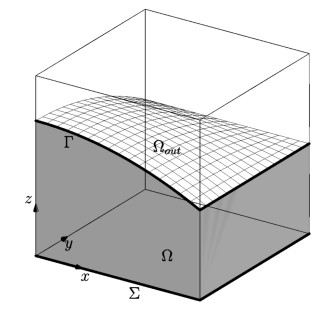
where the index $ (_0) $ refers to the reference/initial configuration. This assumption allows us to replace $ \phi $ and $ \rho_f $ with $ \phi_0 $ and $ \rho_{f0} $ whenever required. We remark that the poromechanics problem is solved only in the physical part of the domain, namely $ \Omega(t) $. A sketch of a domain example is show in Figure 1.
In particular, it is shown that the upper boundary is denoted by $ \Gamma(t) $ and it is free to move. The lower boudary is denoted with $ \Sigma $ and it is fixed. The lateral sides of the domain are $ \partial\Omega(t)\setminus(\Gamma(t)\cup\Sigma) $. Under the small perturbations hypothesis, the poromechanics problem is modeled through the following system of equations:
where $ {\bf{u}} $ is the solid matrix displacement vector with respect to the unloaded reference configuration, represented in Figure 1. The function $ p $ is the pore pressure and the forcing term $ {\bf{f}} $ is the volumetric force due to the mass of the porous medium, namely
being $ \rho_s, \, \rho_f $ the densities of the solid and fluid phases, respectively, $ g $ the standard gravity, $ {\bf{e}}_z $ the unit vector in the vertical direction and $ R(t) $ a ramp function $ R(t) = \frac{\eta}{2} \max [(t + \delta t_{gs} + |t+\delta t_{gs}|), 1] $ where $ \eta $ is a suitable slope coefficient to be defined later on and $ \delta t_{gs} $ is the temporal interval needed to reach the geostatic conditions.
We remind that $ \partial_t $ denotes the standard partial derivative with respect to time in the Eulerian framework. The parameters $ \alpha $, $ M $ and $ K $ are the Biot number, the Biot modulus and the the hydraulic conductivity, respectively. We recall that the hydraulic conductivity is defined as the ratio between the permeability ($ k_s $) and the dynamic viscosity of the fluid ($ \mu_f $), namely $ K = k_s/\mu_f $. To complete the definition of the problem we also assume the linear elasticity behavior for the skeleton. This implies that the stress tensor $ \sigma $, appearing in (2.2), is defined by
where $ \mu $ and $ \lambda $ are the Lamé coefficients and $ \varepsilon({\bf{u}}) $ is the symmetric gradient of the skeleton displacement, defined as
For further details on poromechanics, the interested reader is referred to e.g. [13,14].
For a well-posed problem we must complement the previous governing equations with appropriate boundary and initial conditions. We consider the following,
where $ {\bf{n}} $ is the unit outward normal to the boundary. Concerning the initial condition we consider the basin to be in the reference unloaded state so that $ {\bf{u}} = {\bf{0}} $, $ p = 0 $ enforced at the beginning of simulations $ t = -\delta t_{gs} $. We point out that, as illustrated in Figure 2, by the time $ t = 0 $ the basin has reached the geostatic state characterized by $ {\bf{u}} = {\bf{u}}_{gs} $, $ p = p_{gs} $.
By taking into account the conditions (2.7), (2.8), (2.9), the weak formulation of the problem described in (2.2)–(2.3) reads: for each $ t \in (0, T] $, find $ ({\bf{u}}, p) \in {\bf{V}}(t)\times Q(t) $ such that
where $ {\bf{V}}(t): = \{{\bf{u}} \in (H^1(\Omega(t)))^n \, \mid\, {\bf{u}} \mid_{\Sigma} = {\bf{0}} \} $ and $ Q(t): = \{p \in H^1(\Omega(t)) \, \mid\, p\mid_{\Gamma(t)} = 0 \} $. Here, $ H^1(\Omega) $ denotes the Hilbert subspace of $ L^2(\Omega(t)) $ of functions with first weak derivatives in $ L^2(\Omega(t)) $, $ (\cdot, \cdot) $ is the standard inner product in the space $ L^2(\Omega(t)) $. Equation (2.10) is characterized by the following bilinear forms
The main difficulty of problem (2.10) consists of the time-dependence of the domain and of the functional spaces. We aim at removing this dependence at the level of numerical discretization by casting the discrete problem into the CutFEM framework.
2.2. Numerical discretization based on the cut finite element method
In the cut finite element method, briefly CutFEM, the boundary of the physical domain is represented on a background grid using a level set function. The background grid is also used to approximate the solution of the governing problem. In this framework the boundary conditions are built into the discrete variational formulation, leading to a method that can handle a time varying domain avoiding mesh moving algorithms or re-meshing techniques. A comprehensive review which also cover the implementation aspects of the CutFEM method can be found in [8,19].
Let $ \Omega_\mathcal{T} $ be a bounded computational domain, constant in time, with an interface $ \Gamma(t) $ dividing $ \Omega_\mathcal{T} $ into two non-overlapping subdomains $ \Omega(t) $ and $ \Omega_{out}(t) $, so that $ \overline{\Omega}_\mathcal{T} = \overline{\Omega}(t) \cup \overline{\Omega}_{out}(t) $, as show in Figure 1. The active zone, $ \Omega(t) $, represents the physical domain, while $ \Omega_{out} $ is a fictitious region.
Let $ \mathcal{T}_h: = \{T\} $ denote a triangulation of $ \Omega_\mathcal{T} $, not necessarily conformal to the interface $ \Gamma(t) $. The collection of elements that are intersected by $ \Gamma $ is denoted with $ \Omega_\Gamma: = {T \in \mathcal{T}_h : T \cap \Gamma \neq \emptyset} $.
Let us introduce the discrete spaces
where $ \mathbb{P}^s $ denotes the space of scalar piecewise polynomials of order $ s $.
We consider a decomposition of the finite element spaces $ {\bf{V}}^r_h, \, Q_{h}^s $ as proposed in [28] and also used in [34]. For simplicity, we address the decomposition for $ {\bf{V}}^r_h $ solely, the one for $ Q_{h}^s $ follows similarly. We separate the nodes related to each finite element space into the ones neighboring the interface $ \mathcal{I}^\Gamma ({\bf{V}}_h^r) $ from the remaining ones in the active part of the domain $ \mathcal{I}^\Omega ({\bf{V}}_h^r) $ and those in the fictitious domain $ \mathcal{I}^{\Omega_{out}} ({\bf{V}}_h^r) $. Precisely, let $ \mathcal{I} ({\bf{V}}_h^r) $ be the set of all degrees of freedom of $ {\bf{V}}_h^r $ and let $ \phi_k $ be the corresponding nodal basis functions. The degrees of freedom related to basis functions entirely supported in $ \Omega $ and $ \Omega_{out} $ are $ \mathcal{I}^\Omega ({\bf{V}}_h^r) : = \{k: \ \mbox{supp}(\phi_k) \subset \Omega\} $ and $ \mathcal{I}^{\Omega_{out}} ({\bf{V}}_h^r) : = \{k: \ \mbox{supp}(\phi_k) \subset \Omega_{out}\} $ respectively. Their complementary set is $ \mathcal{I}^\Gamma ({\bf{V}}_h^r) = \mathcal{I} ({\bf{V}}_h^r) \setminus \big(\mathcal{I}^\Omega ({\bf{V}}_h^r) \cup \mathcal{I}^{\Omega_{out}} ({\bf{V}}_h^r) $. Then, we use those sets to construct the following subspaces,
and we decompose the finite element space as $ {\bf{V}}_h^r = {\bf{V}}_{h}^\Gamma \oplus {\bf{V}}_{h}^\Omega \oplus {\bf{V}}_{h}^{\Omega_{out}} $, so that any test function $ {\bf{v}}_h \in{\bf{V}}_h^r $ can be uniquely represented as as $ {\bf{v}}_h = {\bf{v}}_h^\Gamma + {\bf{v}}_h^{\Omega} + {\bf{v}}_h^{\Omega_{out}} $.
The semi-discrete scheme can be written as follows: find $ ({\bf{u}}_h, p_h) \in {\bf{V}}_{h}^r\times Q_{h}^s $ such that:
Since all the integrals are defined either on $ \Omega $ or on $ \Gamma $, it would be equivalent to use test functions defined on $ {\bf{V}}_{h}^\Gamma \oplus {\bf{V}}_{h}^\Omega $ solely. In practice, we find more convenient to use formulation (2.11) and to set the degrees of freedom of $ \mathcal{I}^{\Omega_{out}} ({\bf{V}}_h^r) $ and $ \mathcal{I}^{\Omega_{out}} (Q_h^s) $ to zero.
For the imposition of the pressure constraint in the internal unfitted interface $ \Gamma(t) $ in the second equation of (2.11), we use Nitsche's method following the approaches proposed in the seminal work [20], see also [6,22] for applications of the method to Stokes problem and poromechanics. This technique allows to weakly enforce interface conditions at the discrete level by adding appropriate penalization terms to the variational formulation of the problem. This results in the modified problem formulation,
where $ h $ is the characteristic size of the quasi-uniform computational mesh and $ \gamma > 0 $ denotes a penalization parameter independent on $ h $ and on the parameters of the problem. Finally, we consider a backward-Euler time discretization scheme. Denoting with $ \tau $ the computational time step, the fully discretized problem at time $ t^n $, $ n = 1, 2, ..., N $ reads as follows: find $ ({\bf{u}}^n_h, p^n_h) \in {\bf{V}}_{h}^r\times Q_{h}^s $ such that
for all $ {\bf{v}}_h \in {\bf{V}}_{h}^r $ and $ q_h \in Q_{h}^s $. We notice that the finite element space of $ p_h^{n-1} $ may not coincide with the one of $ q_h $, relative to the current time $ t^n $. To compute the integrals on the right hand side, we project $ p_h^{n-1} $ onto the space $ Q_{h}^\Gamma \oplus Q_{h}^\Omega $, such that the degrees of freedom of the projected $ p_h^{n-1} $ and $ q_h $ are conformal. If $ \mathcal{I}^{\Omega, n-1} (Q_h^s) \cup \mathcal{I}^{\Gamma, n-1} (Q_h^s) \subset \mathcal{I}^{\Omega, n} (Q_h^s) \cup \mathcal{I}^{\Gamma, n} (Q_h^s) $ the projection is just a simple extension to zero of the new active degrees of freedom. Otherwise, we just discard at time $ n $ the degrees of freedom that were active at time $ n-1 $. We finally remark that bilinear forms of problem (2.13) are defined either on $ \Omega $ or $ \Gamma $. As a result the degrees of freedom $ \mathcal{I}^{\Omega_{out}} ({\bf{V}}_h^r), \, \mathcal{I}^{\Omega_{out}} (Q_h^s) $ are not properly constrained. In practice, all the matrix blocks related to these degrees of freedom are set to the identity, with a corresponding null right hand side, such that all the degrees of freedom on $ \Omega_{out} $ are constrained to vanish.
2.3. Fixed-stress splitting
We focus the attention on the solution of the system (2.13) through the fixed stress iterative scheme as presented e.g. in [4,23,26,30] and used in several studies, see for example [1,3,17,33] as a solver and preconditioner for poromechanics problems.
In this algorithm the flow is solved first, followed by the solution of the mechanical problem. At each time step, the procedure is iterated until the solution converges within an acceptable tolerance.
The first step reads as follows: given $ ({\bf{u}}_h^{n, k}, p_h^{n, k}) \in {\bf{V}}_{h}^r\times Q_{h}^s $ find $ p_h^{n, k+1} \in Q_{h}^s $ such that
where $ (\cdot^k) $ denotes the iteration index. The second step of the algorithm reads: given $ p_h^{n, k+1} \in Q_{h}^s $ find $ {\bf{u}}_h^{n, k+1}\in{\bf{V}}_{h}^r $ such that
The iterative steps are performed until the following convergence criterion is fulfilled
where $ \eta_{p} $ and $ \eta_{u} $ are the desired tolerances (here chosen equal to $ 10^{-7} $).
For notational convenience, we reformulate the fixed-stress steps in a more compact form as
We will refer at $ B_p $ and $ B_u $ as the system matrices of the first (pressure) and the second (displacement) step of the fixed-stress algorithm.
The real number $ \beta \ge 0 $ is a stabilization parameter and has to be chosen such that the convergence of the scheme is ensured. We refer to e.g. [23,30] for the choice of $ \beta $ and to [1,4,5,26,31] for a mathematical interpretation and analysis of it. In particular, the optimization of the parameter $ \beta $ is performed in [31]. We remark that all the works mentioned above are referring to classical discretizations of the Biot equations, for the CutFEM method presented in this paper the convergence analysis of the iterative method is thoroughly addressed in Section 3.6.
2.4. Preliminary numerical experiment
In this section we analyze the performance of the original fixed stress algorithm, namely (2.17), in order to investigate the effects of the CutFEM discretization in the solution of the problem. To this purpose we use two computational test cases arising from different choices of the finite element space for the discretization of the displacement. In the first test case we take $ ({\bf{u}}_h, p_h) \in {\bf{V}}_{h}^1\times Q_{h}^1 $ while in the second case we choose $ ({\bf{u}}_h, p_h) \in {\bf{V}}_{h}^2\times Q_{h}^1 $. We consider a cubic computational domain characterized by an edge of $ 4 $ Km. The physical domain is described by the negative part of the following level set function
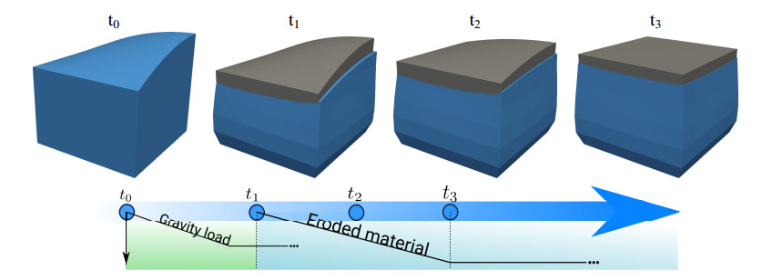
where $ t^+ $ is the physical time in the temporal window $ [0, 4Ky] $ (Ky stands for kilo-years) and $ l $ is the characteristic length of the domain. A sketch of the initial geometry of the physical domain is shown in the top left part of Figure 2, while the material properties considered are reported in Table 1. According to (2.18), $ \Gamma(t) $ is such that in some points $ [x, y] $ the elevation of ground surface decreases as time evolves, while it increases in some other points. With this choice, we aim at demonstrating the capability of the approach to model erosion as well as deposition of material. On a sufficiently large spatial scale, the two phenomena must necessarily take place together, because of mass conservation.
To reach the geostatic condition we consider a temporal interval of $ 3.99 Ky $ in wich the ramp function $ R(t) $, introduced in Eq. (2.4), reads $ R(t) = \frac{\eta}{2} \max [(t + \delta t_{gs} + |t+\delta t_{gs}|), 1] $ with $ \delta t_{gs} = 3.99 Ky $ and $ \eta = (t_r + \delta t_{gs} + |t_r+\delta t_{gs}|)^{-1} $ with $ t_r\approx - 1 Ky $. A schematic of the simulation set up is reported in the timeline in the bottom part of Figure 2. We notice that the simulation is split in three parts: before $ t_1 = 0Ky $, between $ t_1 = 0Ky $ and $ t_3 = 3.99Ky $ and after $ t_3 = 3.99Ky $. The first part from $ t_0 = -\delta t_{gs} $ to $ t_1 $ is used to reach the geostatic condition that are reached at $ t_1 = 0Ky $. The second part of the simulation, namely from $ t_1 = 0Ky $ to $ t_3 = 3.99Ky $ is when the erosion/deposition take place, while between $ t_3 $ and $ t_{end} \approx 8 Ky $ there isn't any change in the basin configuration. We use a time step size of $ 3.15\cdot 10^9 s \approx 0.1 Ky $ so that the simulation requires $ 40 $ time steps for the first, the second and the third part. The level set function is updated just for $ 40 $ time steps after $ t_1 = 0 $ so that remains steady for $ t > t_3 = 3.99Ky $.
The performance of the numerical solver is measured by three indices:
where $ n_{p} $ and $ n_{u} $ are the average number of GMRES iterations needed for the solution of the pressure and the displacement subproblem, namely step 1 and step 2 of (2.17), $ n_{max, {p}} $ and $ n_{max, {u}} $ are the maximum number of iterations for the pressure and the displacement problem respectively, while the number of fixed stress iterations per time step is $ n_{fs} $.
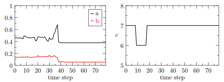
The behavior of $ a $ and $ b $ over time for the case $ ({\bf{u}}_h, p_h) \in {\bf{V}}_{h}^1\times Q_{h}^1 $ is reported in the left part of Figure 3. We notice that the average number of iterations needed for the solution of the pressure and the displacement sub-problem ($ a $ and $ b $ indices) is highly variable and a few peaks can be observed. We remark that the indices $ a $ and $ b $ are related to the convergence rate of GMRES and, as a consequence, to the conditioning of the two sub-problems. Depending on how the level set intersects the computational domain, the two sub-problems may become ill-conditioned and a larger number of iterations is needed for the fixed stress algorithm to converge. In the first test case, we notice that the indices $ a $ and $ b $ do not reach their maximum (unit) value, meaning that the sub-problems are properly solved at every time step. In such condition, as we see from the right panel of Figure 3 ($ c $ index), the number of fixed stress iterations at each time step remains almost constant.
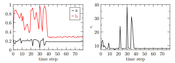
The behavior of the three indices for the test case $ ({\bf{u}}_h, p_h) \in {\bf{V}}_{h}^2\times Q_{h}^1 $ is reported in Figure 4. We notice that the variability of the indices $ a $ and $ b $ is greater that in the previous case and furthermore, at certain time steps, the $ b $ index reaches its maximum. More precisely, the second step of the fixed stress algorithm does not reach convergence. The index $ c $ of Figure 4, shows that the ill-conditioning of the sub-problems affects also the global convergence of the fixed stress algorithm. In particular, we notice that the $ c $ index follows the same trend of $ b $ and severe peaks occur when the solver of the subproblem $ b $ does not converge.
From these preliminary test cases we infer that as long as the sub-problems are accurately solved, the global convergence of the fixed stress algorithm is not significantly affected, while is highly deteriorated when one of the two steps is not properly resolved. Then, the aim of this work is exploring different numerical techniques to overcome the dependence of the sub-problems form the size of cut-elements and, as a consequence, of the fixed stress algorithm from the position of the unfitted interface.
3.
Stability analysis and conditioning of the problem
In this section we investigate the spectral properties of the systems associated to the two steps of the fixed stress algorithm. We show that the CutFEM approximation may cause the ill-conditioning of the sub-problems, depending on how the level set function intersects the computational grid. In the second part of the section, we introduce a stabilization term and a preconditioner that cure the ill-conditioning of the CutFEM approximation method.
3.1. Preliminary results for the analysis of CutFEM
In the CutFEM framework interface conditions are enforced weakly and numerical integration over sub-elements is required. The integrals over very small sub-elements lead to very small element matrix entries and therefore to ill-conditioned systems. Since the introduction of CutFEM various authors have proposed different techniques to avoid this type of ill-conditioning [7,9,10,24,25,28,29,34]. Among this non exhaustive list, we refer to [7], where the ghost penalty stabilization is introduced.
The idea of [7] is to add a penalty term in the interface zone that extends the coercivity of the (physical) operator also in the region of the computational domain where the solution has no physical significance. Let us introduce the following norms for any $ q_h \in Q_h^s $ (for simplicity we use the scalar notation, but these definitions can be straightforwardly extended to vector valued functions)
Following [7] we introduce the following discrete inequalities that will be used in the analysis of the problem:
where the constants $ C_P, \, C_I $ are independent of the size of cut elements. Furthermore, we need estimates of the discrete functions in terms of their degrees of freedom. More precisely, we denote the degrees of freedom of $ q_h \in Q_h^s $ with $ q_h: = \sum_{i = 1}^N q_i \phi_{h, i} $ as $ {\bf{q}}: = \{q_i\}_{i = 1}^N \in \mathbb{R}^N $. Then, there exist constants $ c_{min, 0} $ and $ c_{max, 0} $ such that
When properties of discrete functions are considered on meshes that are cut by the boundary, the smallest size of cut elements may affect the validity such properties. To define the smallest cut element, we assume there exist a node $ x_n $ such that the basis function related to such node have small support in the physical domain, i.e. $ \mbox{meas}_d(\cup_{T:x_n \in T} T \cap \Omega) < < h^d $. Let $ x_h $ be the nodal basis function related to that node. Let $ z_n $ be the node and $ z_h $ be the basis function such that $ \mbox{meas}_d(\cup_{T:z_n \in T} T \cap \Omega)/\mbox{meas}_d(T) $ is minimal among the whole mesh. Then we define the smallest (relative) support of a basis function defined on cut element as
In the case of a mesh cut by the boundary, following [34] and in particular Lemma 3.3 and Lemma 3.4 respectively, for piecewise linear finite elements, namely $ r = 1, \, s = 1 $, and for the special function $ z_h $ related to definition (3.4), we have that there exist constants $ c_{min, 1}, \, c_{min, 2}, \, c_{max, 1}, \, c_{max, 2} $ such that
Finally, in Lemma 3.7 of [34] it is shown that there exists a constant $ C_T $, independent of the mesh cuts, such that for any $ q_h \in Q_h^1 $ it holds,
On the basis of these results, in the following we present the analysis of the two sub-problems of the fixed-stress approach, showing how the interface position affects their conditioning in both the standard and the stabilized formulation.
3.2. Stability analysis of pressure problem
Equation (2.14), with a generic right hand side, can be written in a more compact form as
where
Before proceeding, we observe that using standard arguments based on the norms and the inequalities defined in the previous Section, it is straightforward to prove the following properties of the pressure problem, with constants $ m_c $ and $ M_c $ uniformly independent to the mesh characteristic size and the cut elements,
To study the conditioning of the system matrix associated with (3.8), we address the spectral properties of the matrix $ B_p $ of (2.17). It is the sum of a mass ad a stiffness matrix, namely $ B_p = M+C $. The eigenvalues/eigenfunctions of (3.8), namely $ \vartheta, y_h $ are the solution of the following problem
Introducing a suitable parameter $ C_B $, equation (3.11) can be written as
and, as a consequence, the eigenvalues $ \vartheta $ are related to the eigenvalues $ \zeta $ associated to the operator $ c_h $. For this reason, we study the spectral properties of the matrix associated to (3.12).
Let $ k(C) : = ||C||\, ||C^{-1}|| $ be the condition number of a generic matrix $ C $, where $ ||C||: = \sup_{{\bf{x}}\in \mathbb{R}^N}\frac{|C {\bf{x}}|}{|{\bf{x}}|} $ and $ |\cdot| $ denotes the euclidean norm on $ \mathbb{R}^N $. Let us consider $ {\bf{x}} \in \mathbb{R}^N $, associated to $ x_h \in Q^s_{h} $ such that $ supp(x_h) \subset \Omega $, and therefore $ ||x_h||_{0, \Omega} = ||x_h||_{0, \Omega_{\mathcal{T}}} $. It can be shown, using the coercivity relation (3.9), the Poincaré inequality (3.1) and (3.3) that
We focus now on $ ||C^{-1}|| $. By definition we have
Let us now take the special function $ z_h $ of (3.4),
Using the continuity of the bilinear form (3.10) combined with (3.6) applied to $ z_h $, (3.3) applied to $ w_h $, and reminding that $ |{\bf{z}}| = 1 $ we obtain that
In conclusion we have that
meaning that the conditioning of the pressure sub-problem tends to infinity when $ \nu \rightarrow 0 $.
3.3. A stabilized formulation of the pressure equation
Let $ \mathcal{E}_B $ be the set of element edges in the boundary zone, more precisely,
Following [11], for any $ p_h \mbox{ and } q_h\in Q_{h}^1 $ the ghost penalty stabilization operator $ j(\cdot, \cdot) $ is given by
and Equation (3.8) is modified as follows,
Then, the bilinear form of the stabilized pressure problem is
and we denote by $ G $ the related matrix.
In [7] it is shown that the stabilization operator does not affect the continuity and the coercivity of the problem, such that there exist constants $ m_C, \, M_C $
Using (3.3) and the standard inverse inequality we obtain,
For $ ||G^{-1}|| $ using the coercivity, the inverse inequality and the bound (3.3) we have,
Using the Poincaré type inequality (3.1) and the bound (3.3)
As a result we have
Using the previous inequality we estimate $ ||G^{-1}|| $ as
It follows that $ k(G) = ||G||\, ||G^{-1}|| \simeq h^{-2} $ is not dependent by the smallest cut element. The condition number of $ G $ indeed scales with $ h $ as expected for the standard FEM method.
3.4. Analysis of the displacement sub-problem
We focus on the operator $ a({\bf{u}}, {\bf{v}}) $ defined as
For the upper bound of the bilinear form it can be shown that the following inequalities hold true,
For the lower bound of the bilinear form we have straightforwardly that $ a({\bf{u}}_h, {\bf{u}}_h) \geq m_a || \nabla {\bf{u}}_h ||_{0, \Omega}^2 $. Using Korn's inequality, in particular $ ||{\bf{u}}_h ||_{0, \Omega} \leq C_K ||\nabla {\bf{u}}_h||_{0, \Omega}\, , \forall {\bf{u}}_h \in [H_0^1(\Omega)]^d $, (see for example [16]) we obtain that
We now estimate the condition number of the system matrix $ A $ as $ k(A) = ||A||||A^{-1}|| $. Let us consider $ {\bf{x}}_h \in {\bf{V}}_{h}^1 $ such that $ \mathrm{supp}({\bf{x}}_h)\subset \Omega $. Therefore we have $ || {\bf{x}}_h ||_{0, \Omega} = || {\bf{x}}_h ||_{0, \Omega_{\mathcal{T}}} $. Using this function in the coercivity of $ a(\cdot, \cdot) $ and exploiting the bound (3.3) we obtain
As in the previous case we evaluate $ ||A^{-1}|| $ as
where $ {\bf{z}} $ is the vector of degrees of freedom of the function $ {\bf{z}}_h $ related to (3.5), (3.6). Then, there holds
and then following (3.13) we obtain
The condition number is therefore bounded from below by the constant
We notice that, also in the displacement subproblem, the conditioning of the system matrix depends on the smallest cut element.
3.5. Preconditioning of the displacement sub-problem
We address the second step of the fixed-stress approach (2.17) associated to the linear elasticity problem that reads,
On the basis of the decomposition $ {\bf{V}}_h^r = {\bf{V}}_{h}^\Gamma \oplus {\bf{V}}_{h}^\Omega \oplus {\bf{V}}_{h}^{\Omega_{out}} $, after filtering out the redundant degrees of freedom of $ {\bf{V}}_{h}^{\Omega_{out}} $, the matrix $ B_u $ admits the following block representation,
where
The system (3.23) is naturally ill-conditioned because it consists of an almost incompressible elasticity problem. In addition, the corresponding matrix is assembled on possibly small cut-elements. We simultaneously reduce the stiffness of the system and cure the instability due to the small cut-elements by means of a preconditioner and a stabilization term. Following [34] we assume that the only genuinely stiff block of $ B_u $ is $ B^\Omega_u $. As a result we propose the following preconditioner
We solve the problem of $ B_u $ by means of preconditioned Krylov iteration that requires the inversion of $ P $. The solution of the diagonal lower block sub-system $ \mbox{diag}(B_u^{\Gamma }) $ is trivial, while the inversion of the upper block $ \mbox{diag}(B_u^{\Omega}) $ is computationally demanding. We observe that the latter operation is the solution of a standard linear elasticity problem. We achieve this task by means of an Algebraic Multigrid (AMG) algorithm, which has been successfully used for this class of operators, as discussed in [18].
We also adopt a stabilization operator for the elasticity problem, to ease the ill-conditioning related to the presence of small cut-elements. Following the approach described in section 3.3 we add to equation (2.15) the following ghost penalty operator
where $ \partial^i $ denotes the $ i- $th order derivative and $ \mathcal{E}_B $ is the set of element edges in the boundary zone defined in Eq. (3.14). This is a more general form of the ghost-penalty stabilization operator introduced for the pressure in section 3.3, which can be applied either to linear or quadratic finite elements, namely the case $ {\bf{u}}_h \in {\bf{V}}_h^r $ with $ r = 1 $ and $ 2 $. For a comprehensive review of the ghost penalty stabilization approach we remand the interested reader to [12]. In conclusion, the stabilized form of the displacement sub-problem reads as,
3.6. Analysis of the fixed-stress approach with CutFEM
In this section we investigate the convergence of the fixed stress algorithm in relation with ill-conditioning of the two sub-problems, due to the presence of small cut-elements. For this reason, we address the pressure and elasticity problems of (2.17) in absence of the ghost penalty stabilizations. Anyway, it is easy to see that the same conclusions of this section apply to the stabilized formulation including $ j_p(\cdot, \cdot) $ and $ j_u(\cdot, \cdot) $.
Let us introduce the splitting error of the fixed stress approach as
We subtract the fixed-stress equations form the monolithic problem formulation. The pressure equation becomes
The displacement error equation reads
First, we choose the test function as $ q_h = e_p^k $ and $ {\bf{v}}_h = {\bf{e}}_u^{k-1} $. Equation (3.28) becomes now
while (3.29) gives
Using the polarization identity $ a\cdot b = 1/4(a+b)^2 -1/4(a-b)^2 $ we get
and by the the binomial identity $ (a-b, a) = \frac{1}{2} a^2 + \frac{1}{2}(a-b)^2 - \frac{1}{2}b^2 $ we obtain
Regarding the terms arising from the CutFEM approximation, using (3.7) we obtain,
By choosing $ \delta = \frac{\nu^{1/d}}{C_T} $, $ 1-\frac{\delta}{2} \frac{C_T}{\nu^{1/d}} = \frac{1}{2} $ and $ \gamma = \frac{C_T}{\nu^{1/d}} $ we obtain
Using (3.30), (3.31) (3.32), (3.33), (3.34) and (3.35) we get
Second, we address the terms arising from the splitting error of the displacement problem. From equation (3.31) taken at iteration $ k $ and $ k-1 $ and using the test function $ {\bf{v}}_h = {\bf{e}}_u^{k} - {\bf{e}}_u^{k-1} $, we have
We recall that
Using Cauchy-Schwarz and Young's inequality we obtain,
As a result we have,
Equation (3.38) shows the convergence of the displacement is dominated by the convergence of the pressure. Then, combining inequalities (3.36) and (3.38) we obtain,
which, on the basis of the Banach contraction theorem, proves that $ ||e_p^{k-1}||_{0, \Omega}^2 \rightarrow 0 $, provided that
Finally, owning to the Poincaré inequality, for the splitting error of the pressure we obtain,
showing that the global convergence of the fixed stress algorithm is not affected by the position of the unfitted interface $ \Gamma $, because when $ \nu \rightarrow 0 $ the constant of (3.40) is uniformly bounded. We conclude that as long as the two sub-problems are well posed, in the case of piecewise linear finite elements for the pressure approximation, the global convergence of the fixed stress algorithm depends only on the material properties of the problem and we expect a constant number of fixed stress iteration. This theoretical result is in accordance on what is obtained in the preliminary test case where the $ c $ index remains almost constant as shown in the right part of Figure 3.
4.
Numerical experiments
In this section we investigate the performance of the stabilization term introduced in Section 3.2 and of the preconditioner described in Section 3.5, by means of several numerical experiments. In Test 1 we consider a simple two dimensional problem, because in such simplified configuration the smallest (relative) size of the cut element ($ \nu $) is easily controlled. In the second test, named Test 2, we consider a more realistic three dimensional case.
4.1. Test 1: a two-dimensional problem
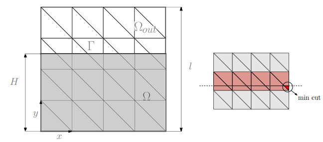
We consider a squared domain as shown in the left part of Figure 5 with a characteristics length $ l = \, 4 $ Km divided into the physical ($ \Omega $) and fictitious region ($ \Omega_{out} $) by the curve $ \Gamma $. The material properties are the ones reported in the right panel of Figure 1. Regarding the boundary conditions, we consider vanishing displacement and null fluid flow on the bottom surface $ y = 0 $, while free stress condition and vanishing pressure are imposed on the remaining faces. The surface $ \Gamma $ is defined as the zero value of the level set function $ \Gamma(y) = y - H $. Using this type of level set function and a uniform triangulation, we control the minimum dimension of the cut element as shown in the right panel of Figure 5.
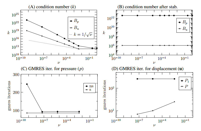
Both the first and the second step of the fixed stress algorithm (2.17) (pressure and displacement step, respectively) are solved by means of GMRES. The number of iterations performed by each step is used to investigate the performance of the pressure stabilization and the preconditioner for the displacement. In Figure 6 (panel A) we show the conditioning of the matrices associated to the fixed-stress sub-problems with respect to the minimum cut-element size. From that figure we notice that the numerical experiments are consistent with the lower bound (dashed line) derived in Section 3. However, we notice that the theoretical bound is not sharp, because when $ \nu $ tends to zero the conditioning of both matrices explode with a rate higher than $ \nu^{-\frac12} $. When the pressure stabilization and the preconditioning of the displacement are applied, the condition number of the pressure and the displacement systems become insensitive to the parameter $ \nu $, as shown in Figure 6 (panel B). The effect of the pressure stabilization term can be seen in Figure 6 (panel C), where we show the number of GMRES iterations needed by the pressure step of the fixed stress algorithm. We notice that the introduction of the stabilization term makes the number of iterations become insensitive to the parameter $ \nu $. Concerning the solver for the displacement, the application of the preconditioner (3.24) requires the inversion of the matrix
In alternative to $ P $, we also consider the diagonal matrix $ P_1 $ defined as
The number of GMRES iterations for the displacement system using these preconditioners, is shown in Figure 6 (Panel D). We notice that both preconditioners optimally cure the stiffness of the matrix due to presence of small cut-elements, because in both cases the convergence rate of GMRES seems to be independent of $ \nu $. However, the full preconditioner $ P $ is more effective, because it highly reduces the number of GMRES iterations.
4.2. Test 2: a three-dimensional numerical experiment
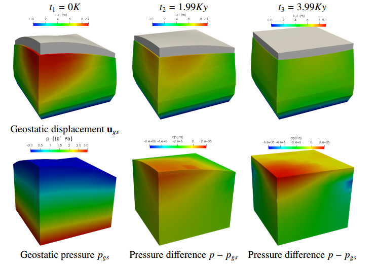
In this section we show and comment the results for a more realistic test case. We consider a tridimensional slab subject to mechanical compaction. The physical domain is described by the intersection of a cube, of edge $ l = 4 $ Km, and the negative part of the level set function defined in (2.18).
A sketch of the physical domain is shown in the top part of Figure 2 at different time steps. We model the slab as a water saturated porous material, characterized by the properties reported in the Table 1. Such parameters are in the range used for modeling sedimentary basins. We remand the interested reader to [2,13,14,27] for further details.
Concerning the boundary conditions we assume that the base of the slab is impermeable and fixed. The lateral surfaces are impermeable, while a free stress condition is imposed for the displacement problem. On the unfitted boundary at the top, we prescribe an homogeneous Dirichlet and an homogeneous Neuman conditions for the pressure and the displacement, respectively. We study the evolution of the slab in a temporal interval as described in Section 2.4. In particular for the second part of the simulation, after the geostatic condition is reached, we investigate the evolution of the slab for $ 8Ky $ using a time step of approximately $ 0.1Ky $. In the top part of Figure 7 we show the displacement field at $ t_1 = 0 $, $ t_2 = 1.99 $ and $ t_3 = 3.99Ky $. The deformed domains (in blue) are obtained warping the current configuration (in gray) by the displacement field magnified by a factor of $ 60 $ so that they can be appreciated. We notice that the displacement field is highly driven by the shape of the physical domain. In particular when the top surface is not planar, the largest deformation occurs in correspondence of the thickest zones of the slab while, in the final part of the simulation when the level set is planar, the displacement field becomes almost constant in the cross section of the slab. Similar considerations also apply to the pressure field, as confirmed by the lower part of Figure 7 where we show the geostatic pressure on the left and the difference between the current and the geostatic pressure at $ t_2 $ and $ t_3 $.
We now investigate the performance of the numerical solver based on the fixed stress algorithm applied to Test 2. In particular we show that the pressure stabilization together with the preconditioning of the elasticity system are effective to reduce the computational cost of the problem. We run numerical experiments for two discretization choices, $ ({\bf{u}}_h, p_h) \in {\bf{V}}_{h}^1\times Q_{h}^1 $ and $ ({\bf{u}}_h, p_h) \in {\bf{V}}_{h}^2\times Q_{h}^1 $.
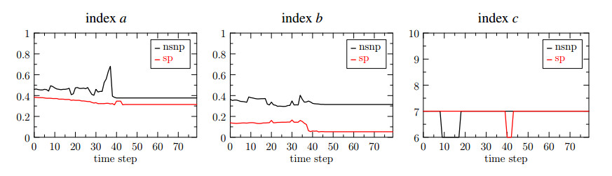
In Figure 8 we show the three indices introduced in Section 2.4, obtained for the case $ (r, s) = (1, 1) $. We compare the performance of the fixed stress algorithm in the original set up (black curves) and using the stabilization term for the pressure problem, namely $ j_p(\cdot, \cdot) $ and the preconditioner $ P $ for the elasticity problem, as described in (3.24) (red curves).
From the index $ a $ we notice that, using the stabilization term the number of iterations for the pressure problem is reduced. Precisely, the peak that occurs near the time step $ 30 $ for the black curve, is no longer present for the red one. Focusing on the index $ b $, we notice that the preconditioner $ P $ effectively reduces the number of iterations needed for the solution of the displacement problem. Finally, from the index $ c $ we see that the number of fixed stress iterations is almost constant both in the original and the stabilized formulation of the problem. This observation supports the conclusions of Section 3.6, confirming that the global convergence of the fixed stress does not depend on the position of the level set, resulting in an almost constant number of iterations.
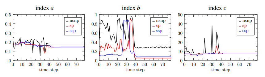
The results obtained in the case of ($ (r, s) = (1, 2) $) are shown in Figure 9. In particular we compare the following cases:
$ (nsnp) $ non stabilized, non preconditioned (black line); it refers to the original formulation of the problem.
$ (sp) $ pressure-stabilized and preconditioned (red line); it refers to the stabilized formulation of the pressure problem and the preconditioner $ P $ for the elasticity problem.
$ (ssp) $ pressure and displacement stabilized and preconditioned (blue line); these data are are obtained using the ghost penalty stabilization $ j_u(\cdot, \cdot) $ in the elasticity problem.
Again, we see that the number of iterations for each subproblem of the fixed stress algorithm decreases for both the sp and ssp cases. Concerning the index $ b $, the overall number of iterations for the displacement significantly lowers in the sp and ssp cases, despite some peaks that are still present. However, the major advantage of using the preconditioner and the stabilization term of the displacement is appreciated from the index $ c $. More precisely, we notice that the peaks of the fixed stress iterations drastically decrease in the sp case and almost vanish in the ssp cases, resulting in a great reduction in the computational cost of the whole coupled system.
5.
Conclusions
In this work we have considered a free-boundary poromechanic problem, relevant for studying the erosion/deposition of a sedimentary basin. The mathematical model for this problem consists of Biot's equations with a moving boundary. We have proposed a discretization method based on CutFEM and the fixed-stress splitting scheme. The use of CutFEM avoids re-meshing the computational domain along with the evolution of the boundary. However, it worsens the conditioning of the matrices in the presence of cut-elements of small size. To overcome this issue, we have introduced a stabilisation term into the problem formulation and used a preconditioner for the numerical solver. Illustrative numerical examples have shown that these numerical techniques are effective and enable the application of the combined CutFEM/fixed stress approach to realistic applications in geomechanics.
Acknowledgments
The authors D.C. and P.Z. acknowledge financial support from ENI S.p.A. The authors F.A.R. and P.Z. thank Equinor for the travel grant through the Akademia program.
Conflict of interest
The authors declare no conflict of interest in this paper.


 DownLoad: