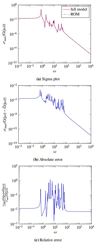
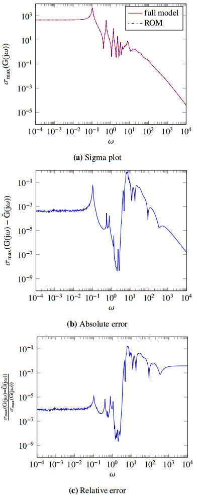
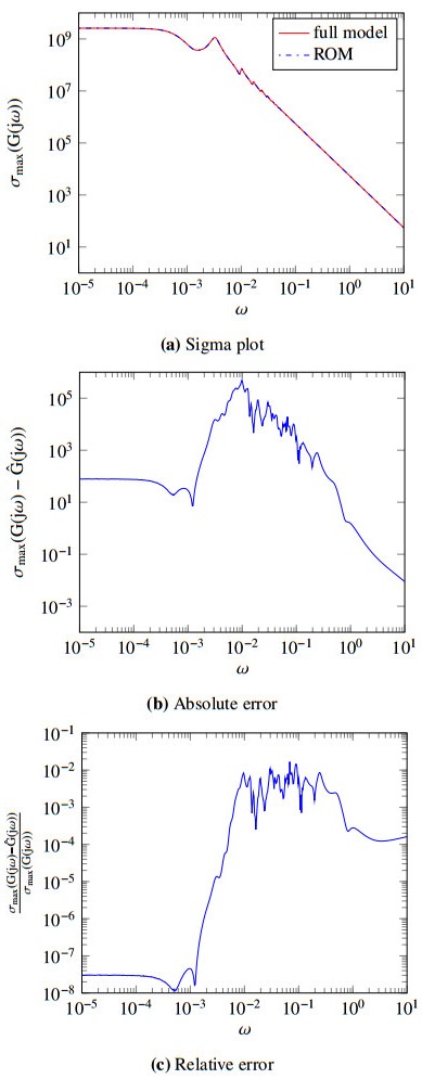
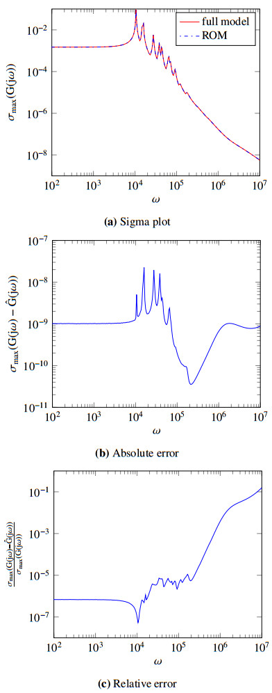
We introduce an efficient structure-preserving model-order reduction technique for the large-scale second-order linear dynamical systems by imposing two-sided projection matrices. The projectors are formed based on the features of the singular value decomposition (SVD) and Krylov-based model-order reduction methods. The left projector is constructed by utilizing the concept of the observability Gramian of the systems and the right one is made by following the notion of the interpolation-based technique iterative rational Krylov algorithm (IRKA). It is well-known that the proficient model-order reduction technique IRKA cannot ensure system stability, and the Gramian based methods are computationally expensive. Another issue is preserving the second-order structure in the reduced-order model. The structure-preserving model-order reduction provides a more exact approximation to the original model with maintaining some significant physical properties. In terms of these perspectives, the proposed method can perform better by preserving the second-order structure and stability of the system with minimized $ \mathcal{H}_2 $-norm. Several model examples are presented that illustrated the capability and accuracy of the introducing technique.
Citation: Md. Motlubar Rahman, Mahtab Uddin, M. Monir Uddin, L. S. Andallah. SVD-Krylov based techniques for structure-preserving reduced order modelling of second-order systems[J]. Mathematical Modelling and Control, 2021, 1(2): 79-89. doi: 10.3934/mmc.2021006
We introduce an efficient structure-preserving model-order reduction technique for the large-scale second-order linear dynamical systems by imposing two-sided projection matrices. The projectors are formed based on the features of the singular value decomposition (SVD) and Krylov-based model-order reduction methods. The left projector is constructed by utilizing the concept of the observability Gramian of the systems and the right one is made by following the notion of the interpolation-based technique iterative rational Krylov algorithm (IRKA). It is well-known that the proficient model-order reduction technique IRKA cannot ensure system stability, and the Gramian based methods are computationally expensive. Another issue is preserving the second-order structure in the reduced-order model. The structure-preserving model-order reduction provides a more exact approximation to the original model with maintaining some significant physical properties. In terms of these perspectives, the proposed method can perform better by preserving the second-order structure and stability of the system with minimized $ \mathcal{H}_2 $-norm. Several model examples are presented that illustrated the capability and accuracy of the introducing technique.

| [1] | V. I. Arnol'd, Mathematical methods of classical mechanics, Springer Science & Business Media, 60 (2013). |
| [2] | R. Riaza, Differential-algebraic systems: analytical aspects and circuit applications, World Scientific, (2008). |
| [3] | M. M. Uddin, Computational Methods for Approximation of Large-scale Dynamical Systems, Chapman and Hall/CRC, (2019). |
| [4] |
M. M. Rahman, M. M. Uddin, L. Andallah, M. Uddin, Tangential interpolatory projections for a class of second-order index-1 descriptor systems and application to mechatronics, Production Engineering, 15 (2021), 9–19. doi: 10.1007/s11740-020-00995-4

|
| [5] | E. Eich-Soellner, C. Führer, Numerical methods in multibody dynamics, Springer, 45 (1998). |
| [6] | R. R. Craig Jr, A. J. Kurdila, Fundamentals of structural dynamics, John Wiley & Sons, (2006). |
| [7] |
B. Yan, S. X.-D. Tan, B. McGaughy, Second-order balanced truncation for passive-order reduction of rlck circuits, IEEE Transactions on Circuits and Systems II: Express Briefs, 55 (2008), 942–946. doi: 10.1109/TCSII.2008.925655
|
| [8] | A. C. Antoulas, Approximation of large-scale dynamical systems, SIAM, (2005). |
| [9] | P. Benner, V. Mehrmann, D. C. Sorensen, Dimension reduction of large-scale systems, Springer, 45 (2005). |
| [10] | M. M. Uddin, Computational methods for model reduction of large-scale sparse structured descriptor systems, (2015). |
| [11] |
B. Moore, Principal component analysis in linear systems: Controllability, observability, and model reduction, IEEE transactions on automatic control, 26 (1981), 17–32. doi: 10.1109/TAC.1981.1102568
|
| [12] |
M. S. Tombs, I. Postlethwaite, Truncated balanced realization of a stable non-minimal state-space system, International Journal of Control, 46 (1987), 1319–1330. doi: 10.1080/00207178708933971
|
| [13] | E. Grimme, Krylov projection methods for model reduction, Ph.D. dissertation, University of Illinois at Urbana Champaign, (1997). |
| [14] |
S. Gugercin, A. C. Antoulas, C. Beattie, H_2 model reduction for large-scale linear dynamical systems, SIAM journal on matrix analysis and applications, 30 (2008), 609–638. doi: 10.1137/060666123
|
| [15] |
S. Gugercin, An iterative svd-krylov based method for model reduction of large-scale dynamical systems, Linear Algebra and its Applications, 428 (2008), 1964–1986. doi: 10.1016/j.laa.2007.10.041
|
| [16] |
F. Tisseur, K. Meerbergen, The quadratic eigenvalue problem, SIAM review, 43 (2001), 235–286. doi: 10.1137/S0036144500381988
|
| [17] | P. Benner, J. Saak, Efficient balancing based mor for second order systems arising in control of machine tools, Proceedings of the MathMod, (2009). |
| [18] | M. S. Hossain, S. G. Omar, A. Tahsin, E. H. Khan, Efficient system reduction modeling of periodic control systems with application to circuit problems, in 2017 4th International Conference on Advances in Electrical Engineering (ICAEE), IEEE, (2017), 259–264. |
| [19] | J.-R. Li, Model reduction of large linear systems via low rank system gramians, Ph.D. dissertation, Massachusetts Institute of Technology, (2000). |
| [20] | S. A. Wyatt, Issues in interpolatory model reduction: Inexact solves, second-order systems and daes, Ph.D. dissertation, Virginia Tech, (2012). |
| [21] | M. Khatibi, H. Zargarzadeh, M. Barzegaran, Power system dynamic model reduction by means of an iterative svd-krylov model reduction method, in 2016 IEEE Power & Energy Society Innovative Smart Grid Technologies Conference (ISGT), IEEE, (2016), 1–6. |
| [22] |
S. Li, J. Trevelyan, Z. Wu, H. Lian, D. Wang, W. Zhang, An adaptive svd–krylov reduced order model for surrogate based structural shape optimization through isogeometric boundary element method, Computer Methods in Applied Mechanics and Engineering, 349 (2019), 312–338. doi: 10.1016/j.cma.2019.02.023
|
| [23] | A. Lu, E. L. Wachspress, Solution of lyapunov equations by alternating direction implicit iteration, Computers & Mathematics with Applications, 21 (1991), 43–58. |
| [24] |
P. Benner, J.-R. Li, T. Penzl, Numerical solution of large-scale lyapunov equations, riccati equations, and linear-quadratic optimal control problems, Numerical Linear Algebra with Applications, 15 (2008), 755–777. doi: 10.1002/nla.622
|
| [25] |
M. M. Rahman, M. M. Uddin, L. S. Andallah, M. Uddin, Interpolatory projection techniques for $\mathcal{H}_2$ optimal structure-preserving model order reduction of second-order systems, Advances in Science, Technology and Engineering Systems Journal, 5 (2020), 715–723. doi: 10.25046/aj050485
|
| [26] | P. Benner, M. Köhler, J. Saak, Sparse-dense sylvester equations in $h_2$-model order reduction, (2011). |
Figures(5) / Tables(2)
Md. Motlubar Rahman, Mahtab Uddin, M. Monir Uddin, L. S. Andallah. SVD-Krylov based techniques for structure-preserving reduced order modelling of second-order systems[J]. Mathematical Modelling and Control, 2021, 1(2): 79-89. doi: 10.3934/mmc.2021006


 DownLoad: