Characterization of the flanking region of the Shiga toxin operon in Stx2a bacteriophages reveals a diversity of the NanS-p sialate O-acetylesterase gene

Stefanía B. Pascal; Ramiro Lorenzo; María Victoria Nieto Farías; John W.A. Rossen; Paula M. A. Lucchesi; Alejandra Krüger; Stefanía B. Pascal; Ramiro Lorenzo; María Victoria Nieto Farías; John W.A. Rossen; Paula M. A. Lucchesi; Alejandra Krüger

doi:10.3934/microbiol.2023030

AIMS Microbiology

2023, Volume 9, Issue 3: 570-590. doi: 10.3934/microbiol.2023030

Previous Article Next Article

Research article

Characterization of the flanking region of the Shiga toxin operon in Stx2a bacteriophages reveals a diversity of the NanS-p sialate O-acetylesterase gene

1.
Universidad Nacional del Centro de la Provincia de Buenos Aires (UNCPBA), Facultad de Ciencias Veterinarias, CISAPA, Tandil, Buenos Aires, Argentina
2.
Centro de Investigación Veterinaria de Tandil (CIVETAN), UNCPBA-CICPBA-CONICET, Tandil, Buenos Aires, Argentina
3.
Laboratory of Neurophysiology, ULB Neuroscience Institute, Université Libre de Bruxelles (ULB), Brussels, Belgium
4.
Laboratory of Medical Microbiology and Infectious Diseases, Isala Hospital, Zwolle, The Netherlands
5.
Department of Medical Microbiology and Infection Prevention, University of Groningen, University Medical Center Groningen, Groningen, The Netherlands

Received: 05 June 2023 Revised: 18 July 2023 Accepted: 20 July 2023 Published: 02 August 2023

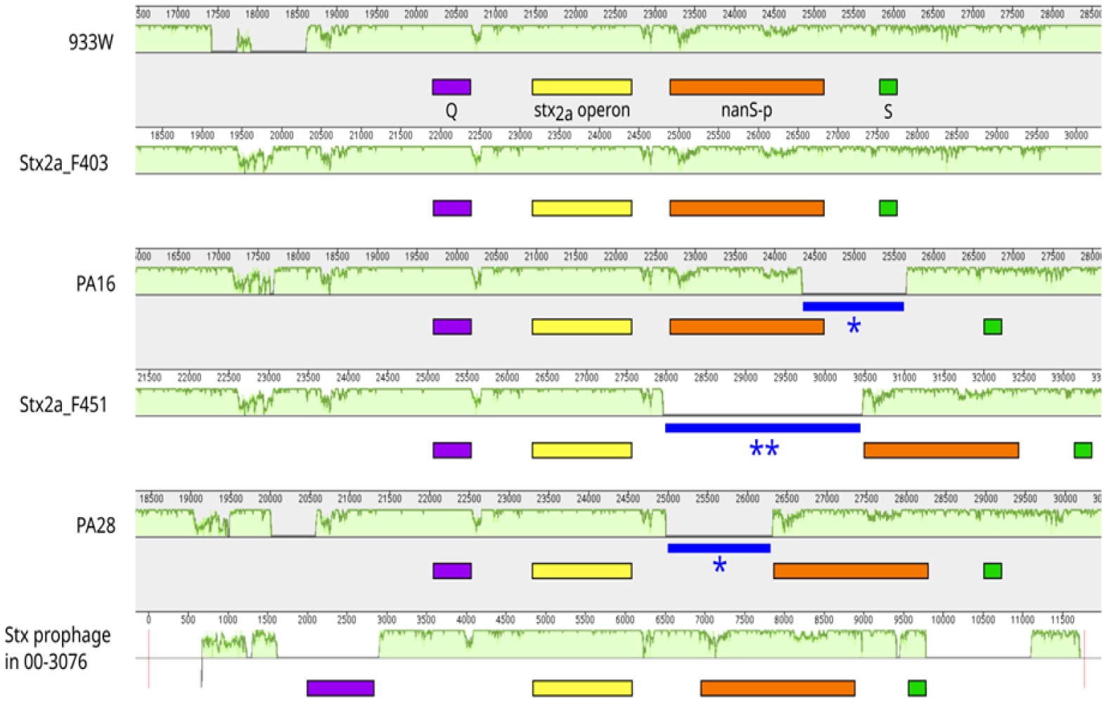
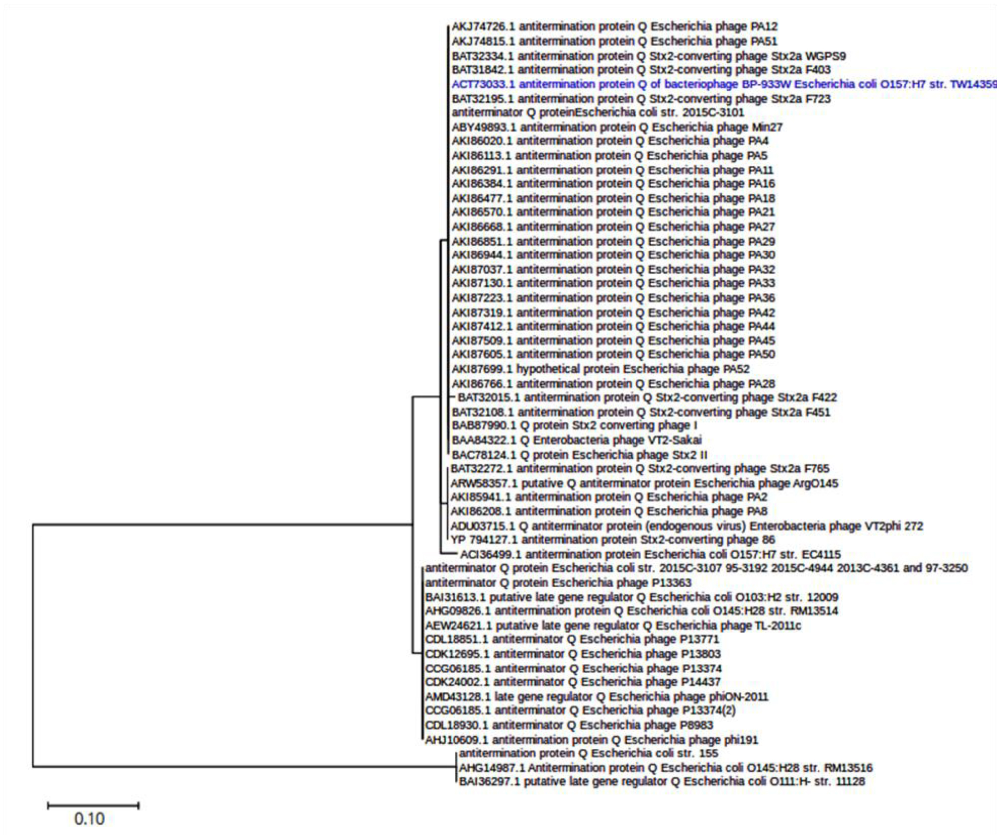
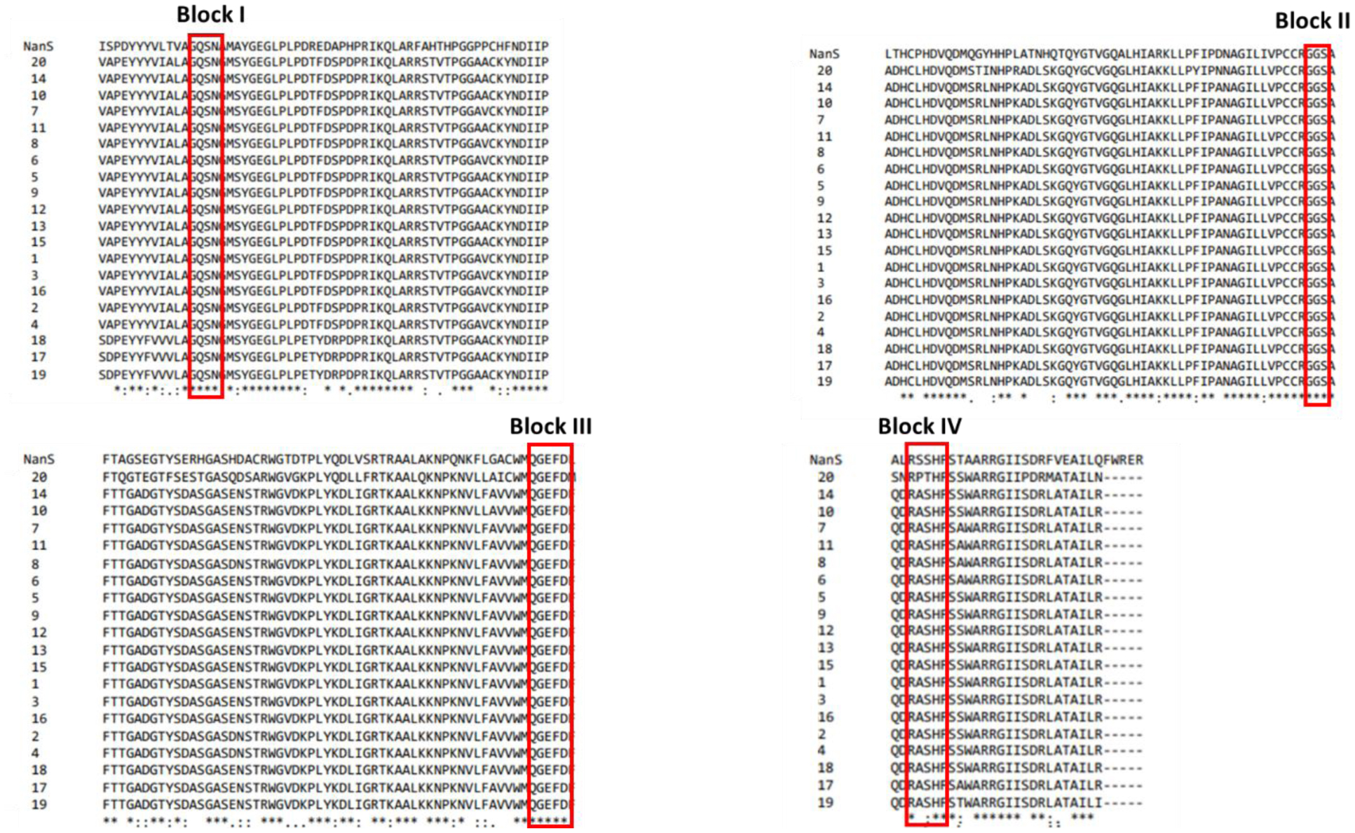
Shiga toxin-producing E. coli (STEC) are diarrheagenic strains that can cause bloody diarrhea and hemolytic-uremic syndrome. Their main virulence factor, the Shiga toxin (Stx), is encoded by phages integrated into the bacterial chromosome. Stx phages are widely diverse and carry many genes with limited or unknown function. As the toxin subtype Stx2a is associated with highly pathogenic strains, this study was mainly focused on the characterization of the stx flanking region of Stx2a phages. Of particular interest was a sialate O-acetylesterase (NanS-p), which has been described previously to be encoded downstream stx in some phage genomes and may confer a growth advantage for STEC. Complete DNA sequences of Stx2a phages and prophages were retrieved from the GenBank database, and the genomic regions from anti-terminator Q to holin S genes were bioinformatically analyzed. Predicted NanSp sequences from phages encoding other Stx subtypes were also studied. Additionally, expression of nanS-p was quantified by qPCR in strains selected from our laboratory collection. The analysis of Stx2a phage genomes showed that all carried the Q, stx_2a, nanS-p and S genes, but with allele diversity and other sequence differences. In particular, sequence differences were detected in each of the three domains of NanS-p esterases encoded by Stx2a phages and other Stx phages; however, nanS-p was not identified in the Stx2e, Stx2f and Stx2g phages analyzed. The expression of nanS-p increased in most stx_2a-positive strains under phage inducing conditions, as was previously shown for stx_2a. As the present work showed diversity at the Q-S region among Stx phages, and particularly in the encoded NanS-p enzyme, future studies will be necessary to evaluate if NanS-p variants differ in their activity and to assess the impact of the absence of nanS-p in certain Stx phages.
- Shiga toxin,
- Stx subtypes,
- phage,
- sialate O-acetylesterase,
- late genomic region,
- diversity
Citation: Stefanía B. Pascal, Ramiro Lorenzo, María Victoria Nieto Farías, John W.A. Rossen, Paula M. A. Lucchesi, Alejandra Krüger. Characterization of the flanking region of the Shiga toxin operon in Stx2a bacteriophages reveals a diversity of the NanS-p sialate O-acetylesterase gene[J]. AIMS Microbiology, 2023, 9(3): 570-590. doi: 10.3934/microbiol.2023030

Related Papers:

Abstract

Shiga toxin-producing E. coli (STEC) are diarrheagenic strains that can cause bloody diarrhea and hemolytic-uremic syndrome. Their main virulence factor, the Shiga toxin (Stx), is encoded by phages integrated into the bacterial chromosome. Stx phages are widely diverse and carry many genes with limited or unknown function. As the toxin subtype Stx2a is associated with highly pathogenic strains, this study was mainly focused on the characterization of the stx flanking region of Stx2a phages. Of particular interest was a sialate O-acetylesterase (NanS-p), which has been described previously to be encoded downstream stx in some phage genomes and may confer a growth advantage for STEC. Complete DNA sequences of Stx2a phages and prophages were retrieved from the GenBank database, and the genomic regions from anti-terminator Q to holin S genes were bioinformatically analyzed. Predicted NanSp sequences from phages encoding other Stx subtypes were also studied. Additionally, expression of nanS-p was quantified by qPCR in strains selected from our laboratory collection. The analysis of Stx2a phage genomes showed that all carried the Q, stx_2a, nanS-p and S genes, but with allele diversity and other sequence differences. In particular, sequence differences were detected in each of the three domains of NanS-p esterases encoded by Stx2a phages and other Stx phages; however, nanS-p was not identified in the Stx2e, Stx2f and Stx2g phages analyzed. The expression of nanS-p increased in most stx_2a-positive strains under phage inducing conditions, as was previously shown for stx_2a. As the present work showed diversity at the Q-S region among Stx phages, and particularly in the encoded NanS-p enzyme, future studies will be necessary to evaluate if NanS-p variants differ in their activity and to assess the impact of the absence of nanS-p in certain Stx phages.

Acknowledgments

Authors thank the technical assistance of M.R. Ortiz. This work was supported by grants from the National Scientific and Technical Research Council of Argentina (CONICET, PIP 0912 and PUE-CIVETAN), Fondo para la Investigación Científica y Tecnológica (FONCYT, PICT-2018-03245) and Secretaría de Ciencia, Arte y Tecnología-Universidad Nacional del Centro de la Provincia de Buenos Aires (SECAT-UNICEN, 03/H312). S.B.P. holds a fellowship from CONICET.

Conflict of interest

The authors declare no conflict of interest.

Use of AI tools declaration

The authors declare they have not used Artificial Intelligence (AI) tools in the creation of this article.

References

[1]	Kaper JB, Nataro JP, Mobley HLT (2004) Pathogenic Escherichia coli. Nat Rev Microbiol 2: 123-140. https://doi.org/10.1038/nrmicro818
[2]	Brzuszkiewicz E, Gottschalk G, Ron E, et al. (2009) Adaptation of pathogenic E. coli to various niches: genome flexibility is the key. Microbial Pathogenomics. Basel: KARGER 110-125. https://doi.org/10.1159/000235766
[3]	EFSA BIOHAZ Panel, Koutsoumanis K, Allende A, et al. (2020) Pathogenicity assessment of Shiga toxin-producing Escherichia coli (STEC) and the public health risk posed by contamination of food with STEC. EFSA J 18: e05967. https://doi.org/10.2903/j.efsa.2020.5967
[4]	Lee MS, Koo S, Jeong D, et al. (2016) Shiga toxins as multi-functional proteins: induction of host cellular stress responses, role in pathogenesis and therapeutic applications. Toxins (Basel) 8: 77. https://doi.org/10.3390/toxins8030077
[5]	Melton-Celsa AR (2014) Shiga toxin (Stx) classification, structure, and function. Microbiol Spectr 2. https://doi.org/10.1128/microbiolspec.EHEC-0024-2013
[6]	Krüger A, Lucchesi PMA (2015) Shiga toxins and stx phages: Highly diverse entities. Microbiol (United Kingdom) 161: 451-462. https://doi.org/10.1099/mic.0.000003
[7]	Pinto G, Sampaio M, Dias O, et al. (2021) Insights into the genome architecture and evolution of Shiga toxin encoding bacteriophages of Escherichia coli. BMC Genomics 22: 366. https://doi.org/10.1186/s12864-021-07685-0
[8]	Mondal SI, Islam MR, Sawaguchi A, et al. (2016) Genes essential for the morphogenesis of the Shiga toxin 2-transducing phage from Escherichia coli O157:H7. Sci Rep 6: 39036. https://doi.org/10.1038/srep39036
[9]	Llarena AK, Aspholm M, O'Sullivan K, et al. (2021) Replication region analysis reveals non-lambdoid Shiga toxin converting bacteriophages. Front Microbiol 12: 640945. https://doi.org/10.3389/fmicb.2021.640945
[10]	Rodríguez-Rubio L, Haarmann N, Schwidder M, et al. (2021) Bacteriophages of Shiga toxin-producing Escherichia coli and their contribution to pathogenicity. Pathogens 10. https://doi.org/10.3390/pathogens10040404
[11]	Smith DL, Rooks DJ, Fogg PC, et al. (2012) Comparative genomics of Shiga toxin encoding bacteriophages. BMC Genomics 13: 311. https://doi.org/10.1186/1471-2164-13-311
[12]	Krüger A, Burgán J, Friedrich AW, et al. (2018) ArgO145, a Stx2a prophage of a bovine O145:H- STEC strain, is closely related to phages of virulent human strains. Infect Genet Evol 60: 126-132. https://doi.org/10.1016/j.meegid.2018.02.024
[13]	Steyert SR, Sahl JW, Fraser CM, et al. (2012) Comparative genomics and stx phage characterization of LEE-negative Shiga toxin-producing Escherichia coli. Front Cell Infect Microbiol 2: 133. https://doi.org/10.3389/fcimb.2012.00133
[14]	Schmidt H (2001) Shiga-toxin-converting bacteriophages. Res Microbiol 152: 687-695. https://doi.org/10.1016/s0923-2508(01)01249-9
[15]	Wagner PL, Neely MN, Zhang X, et al. (2001) Role for a phage promoter in Shiga toxin 2 expression from a pathogenic Escherichia coli strain. J Bacteriol 183: 2081-2085. https://doi.org/10.1128/jb.183.6.2081-2085.2001
[16]	Yin S, Rusconi B, Sanjar F, et al. (2015) Escherichia coli O157:H7 strains harbor at least three distinct sequence types of Shiga toxin 2a-converting phages. BMC Genomics 16: 733. https://doi.org/10.1186/s12864-015-1934-1
[17]	Delannoy S, Mariani-Kurkdjian P, Webb HE, et al. (2017) The mobilome; a major contributor to Escherichia coli stx2-positive O26:H11 strains intra-serotype diversity. Front Microbiol 8: 1625. https://doi.org/10.3389/fmicb.2017.01625
[18]	Nakamura K, Murase K, Sato MP, et al. (2020) Differential dynamics and impacts of prophages and plasmids on the pangenome and virulence factor repertoires of Shiga toxin-producing Escherichia coli O145:H28. Microb Genomics 6. https://doi.org/10.1099/mgen.0.000323
[19]	Rasko DA, Rosovitz MJ, Myers GSA, et al. (2008) The pangenome structure of Escherichia coli: comparative genomic analysis of E. coli commensal and pathogenic isolates. J Bacteriol 190: 6881-6893. https://doi.org/10.1128/JB.00619-08
[20]	Su LK, Lu CP, Wang Y, et al. (2010) Lysogenic infection of a Shiga toxin 2-converting bacteriophage changes host gene expression, enhances host acid resistance and motility. Mol Biol 44. https://doi.org/10.1134/s0026893310010085
[21]	Holt GS, Lodge JK, McCarthy AJ, et al. (2017) Shigatoxin encoding Bacteriophage φ24B modulates bacterial metabolism to raise antimicrobial tolerance. Sci Rep 7: 40424. https://doi.org/10.1038/srep40424
[22]	Veses-Garcia M, Liu X, Rigden DJ, et al. (2015) Transcriptomic Analysis of Shiga-Toxigenic Bacteriophage Carriage Reveals a Profound Regulatory Effect on Acid Resistance in Escherichia coli. Appl Environ Microbiol 81: 8118-8125. https://doi.org/10.1128/AEM.02034-15
[23]	Berger P, Kouzel IU, Berger M, et al. (2019) Carriage of Shiga toxin phage profoundly affects Escherichia coli gene expression and carbon source utilization. BMC Genomics 20: 504. https://doi.org/10.1186/s12864-019-5892-x
[24]	Mitsunaka S, Sudo N, Sekine Y (2018) Lysogenisation of Shiga toxin-encoding bacteriophage represses cell motility. J Gen Appl Microbiol 64: 34-41. https://doi.org/10.2323/jgam.2017.05.001
[25]	Saile N, Voigt A, Kessler S, et al. (2016) Escherichia coli O157:H7 strain EDL933 harbors multiple functional prophage-associated genes necessary for the utilization of 5- N -acetyl-9- O -acetyl neuraminic acid as a growth substrate. Appl Environ Microbiol 82: 5940-5950. https://doi.org/10.1128/AEM.01671-16
[26]	Saile N, Schwarz L, Eißenberger K, et al. (2018) Growth advantage of Escherichia coli O104:H4 strains on 5- N -acetyl-9- O -acetyl neuraminic acid as a carbon source is dependent on heterogeneous phage-Borne nanS-p esterases. Int J Med Microbiol 308: 459-468. https://doi.org/10.1016/j.ijmm.2018.03.006
[27]	McGinnis S, Madden TL (2004) BLAST: at the core of a powerful and diverse set of sequence analysis tools. Nucleic Acids Res 32. https://doi.org/10.1093/nar/gkh435
[28]	Arndt D, Grant JR, Marcu A, et al. (2016) PHASTER: a better, faster version of the PHAST phage search tool. Nucleic Acids Res 4. https://doi.org/10.1093/nar/gkw387
[29]	Joensen KG, Scheutz F, Lund O, et al. (2014) Real-time whole-genome sequencing for routine typing, surveillance, and outbreak detection of verotoxigenic Escherichia coli. J Clin Microbiol 52: 1501-1510. https://doi.org/10.1128/JCM.03617-13
[30]	Siguier P, Perochon J, Lestrade L, et al. (2006) ISfinder: the reference centre for bacterial insertion sequences. Nucleic Acids Res 34: D32-D36. https://doi.org/10.1093/nar/gkj014
[31]	Marchler-Bauer A, Derbyshire MK, Gonzales NR, et al. (2015) CDD: NCBI's conserved domain database. Nucleic Acids Res 43: D222-D226. https://doi.org/10.1093/nar/gku1221
[32]	Jones P, Binns D, Chang HY, et al. (2014) InterProScan 5: genome-scale protein function classification. Bioinformatics 30: 1236-1240. https://doi.org/10.1093/bioinformatics/btu031
[33]	Saier MHJ, Tran C V, Barabote RD (2006) TCDB: the Transporter Classification Database for membrane transport protein analyses and information. Nucleic Acids Res 34: D181-D186. https://doi.org/10.1093/nar/gkj001
[34]	Darling AE, Mau B, Perna NT (2010) progressiveMauve: multiple genome alignment with gene gain, loss and rearrangement. PLoS One 5: e11147. https://doi.org/10.1371/journal.pone.0011147
[35]	Kumar S, Stecher G, Tamura K (2016) MEGA7: molecular evolutionary genetics analysis version 7.0 for bigger datasets. Mol Biol Evol 33: 1870-1874. https://doi.org/10.1093/molbev/msw054
[36]	Sievers F, Wilm A, Dineen D, et al. (2011) Fast, scalable generation of high-quality protein multiple sequence alignments using Clustal Omega. Mol Syst Biol 7: 539. https://doi.org/10.1038/msb.2011.75
[37]	Burgán J, Krüger A, Lucchesi PMA (2020) Comparable stx_2a expression and phage production levels between Shiga toxin-producing Escherichia coli strains from human and bovine origin. Zoonoses Public Health 67: 44-53. https://doi.org/10.1111/zph.12653
[38]	de Sablet T, Bertin Y, Vareille M, et al. (2008) Differential expression of stx₂ variants in Shiga toxin-producing Escherichia coli belonging to seropathotypes A and C. Microbiology 154: 176-186. https://doi.org/10.1099/mic.0.2007/009704-0
[39]	Pfaffl MW (2001) A new mathematical model for relative quantification in real-time RT-PCR. Nucleic Acids Res 29: e45. https://doi.org/10.1093/nar/29.9.e45
[40]	Scheutz F, Teel LD, Beutin L, et al. (2012) Multicenter evaluation of a sequence-based protocol for subtyping Shiga toxins and standardizing Stx nomenclature. J Clin Microbiol 50: 2951-2963. https://doi.org/10.1128/JCM.00860-12
[41]	Tyler JS, Beeri K, Reynolds JL, et al. (2013) Prophage induction is enhanced and required for renal disease and lethality in an EHEC mouse model. PLoS Pathog 9: e1003236. https://doi.org/10.1371/journal.ppat.1003236
[42]	Balasubramanian S, Osburne MS, BrinJones H, et al. (2019) Prophage induction, but not production of phage particles, is required for lethal disease in a microbiome-replete murine model of enterohemorrhagic E. coli infection. PLoS Pathog 15: e1007494. https://doi.org/10.1371/journal.ppat.1007494
[43]	EFSA Panel BH (BIOHAZ).Scientific Opinion on VTEC-seropathotype and scientific criteria regarding pathogenicity assessment. EFSA J (2013) 11: 3138. https://doi.org/10.2903/j.efsa.2013.3138
[44]	Fuller CA, Pellino CA, Flagler MJ, et al. (2011) Shiga toxin subtypes display dramatic differences in potency. Infect Immun 79: 1329-1337. https://doi.org/10.1128/IAI.01182-10
[45]	Forde BM, McAllister LJ, Paton JC, et al. (2019) SMRT sequencing reveals differential patterns of methylation in two O111:H- STEC isolates from a hemolytic uremic syndrome outbreak in Australia. Sci Rep 9: 9436. https://doi.org/10.1038/s41598-019-45760-5
[46]	Fagerlund A, Aspholm M, Węgrzyn G, et al. (2022) High diversity in the regulatory region of Shiga toxin encoding bacteriophages. BMC Genomics 23: 230. https://doi.org/10.1186/s12864-022-08428-5
[47]	Shaaban S, Cowley LA, McAteer SP, et al. (2016) Evolution of a zoonotic pathogen: investigating prophage diversity in enterohaemorrhagic Escherichia coli O157 by long-read sequencing. Microb Genomics 2: e000096. https://doi.org/10.1099/mgen.0.000096
[48]	Scheutz F (2014) Taxonomy Meets Public Health: The case of Shiga toxin-producing Escherichia coli. Microbiol Spectr 2. https://doi.org/10.1128/microbiolspec.EHEC-0019-2013
[49]	Lejeune JT, Abedon ST, Takemura K, et al. (2004) Human Escherichia coli O157:H7 genetic marker in isolates of bovine origin. Emerg Infect Dis 10: 1482-1485. https://doi.org/10.3201/eid1008.030784
[50]	Olavesen KK, Lindstedt BA, Løbersli I, et al. (2016) Expression of Shiga toxin 2 (Stx2) in highly virulent Stx-producing Escherichia coli (STEC) carrying different anti-terminator (q) genes. Microb Pathog 97: 1-8. https://doi.org/10.1016/j.micpath.2016.05.010
[51]	Løbersli I, Haugum K, Lindstedt BA (2012) Rapid and high resolution genotyping of all Escherichia coli serotypes using 10 genomic repeat-containing loci. J Microbiol Methods 88: 134-139. https://doi.org/10.1016/j.mimet.2011.11.003
[52]	Cahill J, Young R (2019) Phage lysis: multiple genes for multiple barriers. Adv Virus Res 103: 33-70. https://doi.org/10.1016/bs.aivir.2018.09.003
[53]	Pang T, Savva C, Fleming K, et al. (2009) Structure of the lethal phage pinhole. Proc Natl Acad Sci U S A 106: 18966-18971. https://doi.org/10.1073/pnas.0907941106
[54]	Nübling S, Eisele T, Stöber H, et al. (2014) Bacteriophage 933W encodes a functional esterase downstream of the Shiga toxin 2a operon. Int J Med Microbiol 304: 269-274. https://doi.org/10.1016/j.ijmm.2013.10.008
[55]	Unkmeir A, Schmidt H (2000) Structural analysis of phage-borne stx genes and their flanking sequences in Shiga toxin-producing Escherichia coli and Shigella dysenteriae Type 1 Strains. Infect Immun 68: 4856-4864. https://doi.org/10.1128/iai.68.9.4856-4864.2000
[56]	Vimr ER (2013) Unified theory of bacterial sialometabolism: how and why bacteria metabolize host sialic acids. ISRN Microbiol 2013: 1-26. https://doi.org/10.1155/2013/816713
[57]	Amigo N, Zhang Q, Amadio A, et al. (2016) Overexpressed proteins in hypervirulent clade 8 and clade 6 Strains of Escherichia coli O157:H7 compared to E. coli O157:H7 EDL933 clade 3 Strain. PLoS One 11: e0166883. https://doi.org/10.1371/journal.pone.0166883
[58]	Polzin S, Huber C, Eylert T, et al. (2013) Growth media simulating ileal and colonic environments affect the intracellular proteome and carbon fluxes of Enterohemorrhagic Escherichia coli O157:H7 strain EDL933. Appl Environ Microbiol 79: 3703-3715. https://doi.org/10.1128/AEM.00062-13
[59]	Herold S, Siebert J, Huber A, et al. (2005) Global expression of prophage genes in Escherichia coli O157:H7 strain EDL933 in response to norfloxacin. Antimicrob Agents Chemother 49: 931-944. https://doi.org/10.1128/aac.49.3.931-944.2005
[60]	Feuerbaum S, Saile N, Pohlentz G, et al. (2018) De-O-Acetylation of mucin-derived sialic acids by recombinant NanS-p esterases of Escherichia coli O157:H7 strain EDL933. Int J Med Microbiol 308: 1113-1120. https://doi.org/10.1016/j.ijmm.2018.10.001
[61]	Franke B, Veses-Garcia M, Diederichs K, et al. (2020) Structural annotation of the conserved carbohydrate esterase vb_24B_21 from Shiga toxin-encoding bacteriophage Φ24B. J Struct Biol 212: 107596. https://doi.org/10.1016/j.jsb.2020.107596
[62]	Jones DT, Taylor WR, Thornton JM (1992) The rapid generation of mutation data matrices from protein sequences. Comput Appl Biosci 8: 275-282. https://doi.org/10.1093/bioinformatics/8.3.275
[63]	Kumar S, Stecher G, Li M, et al. (2018) MEGA X: molecular evolutionary genetics analysis across computing platforms. Mol Biol Evol 35: 1547-1549. https://doi.org/10.1093/molbev/msy096
[64]	Schwartz RM (1978) Matrices for detecting distant relationships. Atlas protein Seq Struct : 353-359.

microbiol-09-03-030-s001.pdf

Reader Comments

Your name:*

Email:*
© 2023 the Author(s), licensee AIMS Press. This is an open access article distributed under the terms of the Creative Commons Attribution License (http://creativecommons.org/licenses/by/4.0)