Telehealth services became commonplace during the COVID-19 pandemic and were widely reported to improve access to medical care in a variety of settings. The primary aim of this study was to assess patient- and provider-reported satisfaction with telehealth services within a multidisciplinary outpatient program for children with feeding disorders.
Caregivers and healthcare providers who participated in telehealth multidisciplinary visits within an outpatient pediatric feeding disorders clinic between April and June 2020 completed an online survey that assessed their visit satisfaction. The visit completion rates of in-person 2019 and virtual 2020 visits were compared.
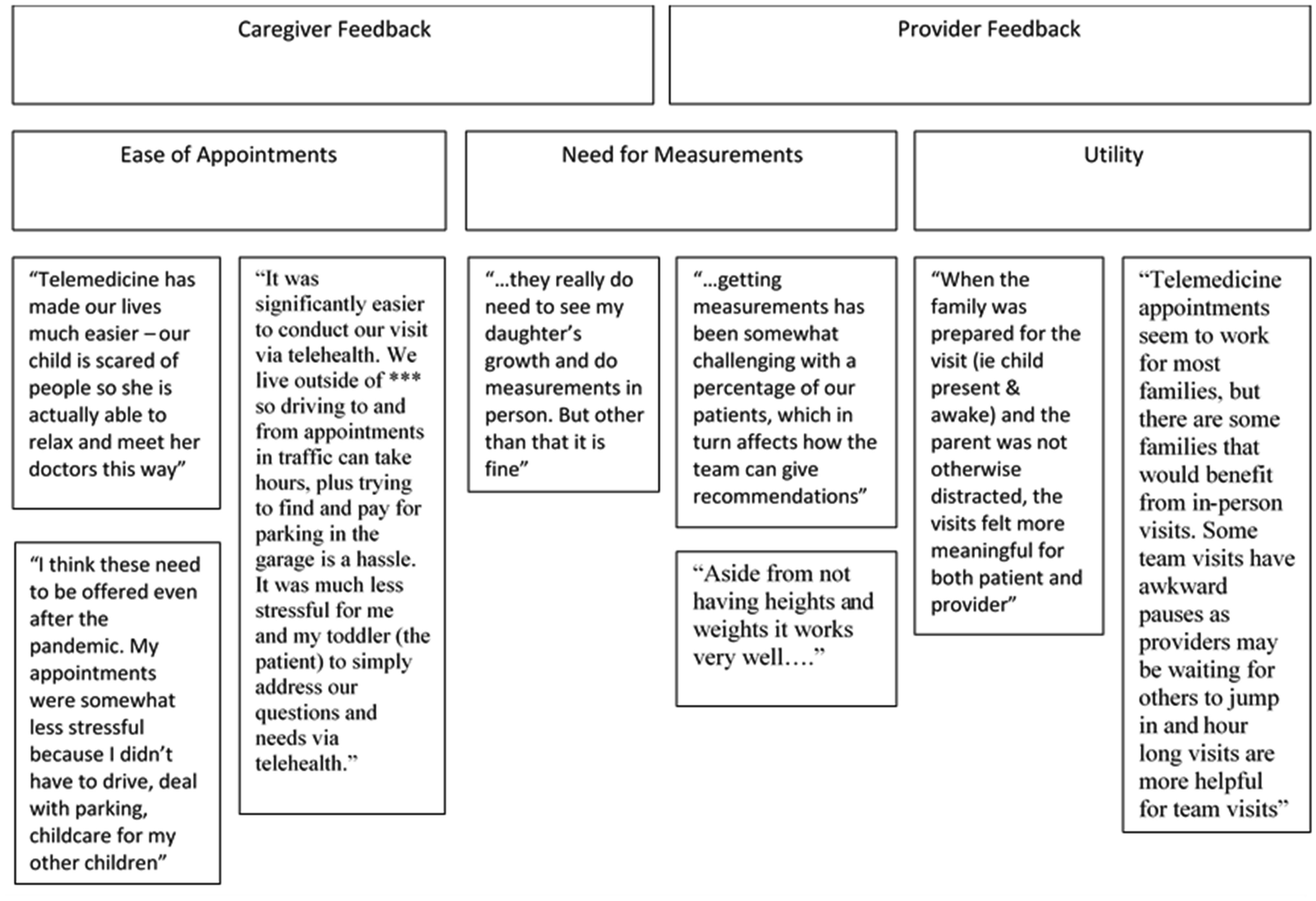
Thirty-six caregivers of children between 1-month and 8-years-old completed the survey. Caregivers indicated their overall satisfaction with telehealth services, finding it more convenient than seeing specialists in person. Caregivers demonstrated interest in continuing telehealth visits. Providers indicated being satisfied with the telehealth visits, with many noting that they were as effective as in-person visits. There was an increase in the number of in-person visits between 2019 compared to virtual visits in 2020, though there were no differences for the visit completion rates.
Both caregivers and providers were satisfied with the telehealth services and highlighted various benefits in response to open-ended questions. However, there were concerns with the lack of available anthropometric data and measurements. Although there were no differences in the no-show rates following the implementation of telehealth, there was a significant increase in the total number of completed visits. Telehealth visits are a crucial resource for caregivers and providers in multidisciplinary pediatric feeding clinics, yet enhancing anthropometric measurements is necessary to provide quality care.
Citation: Ryan D. Davidson, Rebecca Kramer, Sarah Fleet. Satisfaction of telehealth implementation in a pediatric feeding clinic[J]. AIMS Medical Science, 2024, 11(2): 124-136. doi: 10.3934/medsci.2024011
Telehealth services became commonplace during the COVID-19 pandemic and were widely reported to improve access to medical care in a variety of settings. The primary aim of this study was to assess patient- and provider-reported satisfaction with telehealth services within a multidisciplinary outpatient program for children with feeding disorders.
Caregivers and healthcare providers who participated in telehealth multidisciplinary visits within an outpatient pediatric feeding disorders clinic between April and June 2020 completed an online survey that assessed their visit satisfaction. The visit completion rates of in-person 2019 and virtual 2020 visits were compared.
Thirty-six caregivers of children between 1-month and 8-years-old completed the survey. Caregivers indicated their overall satisfaction with telehealth services, finding it more convenient than seeing specialists in person. Caregivers demonstrated interest in continuing telehealth visits. Providers indicated being satisfied with the telehealth visits, with many noting that they were as effective as in-person visits. There was an increase in the number of in-person visits between 2019 compared to virtual visits in 2020, though there were no differences for the visit completion rates.
Both caregivers and providers were satisfied with the telehealth services and highlighted various benefits in response to open-ended questions. However, there were concerns with the lack of available anthropometric data and measurements. Although there were no differences in the no-show rates following the implementation of telehealth, there was a significant increase in the total number of completed visits. Telehealth visits are a crucial resource for caregivers and providers in multidisciplinary pediatric feeding clinics, yet enhancing anthropometric measurements is necessary to provide quality care.
Coronavirus disease 2019
Doctor of medicine
Nurse practitioner
Certificate of clinical competence in speech-language pathology
Certified lactation counselor
Doctor of philosophy
Research Electronic Data Capture
Speech Language Pathologist
Mean
Standard deviation

| [1] |
De Simone S, Franco M, Servillo G, et al. (2022) Implementations and strategies of telehealth during COVID-19 outbreak: a systematic review. BMC Health Serv Res 22: 833. https://doi.org/10.1186/s12913-022-08235-4 
|
| [2] | Bhatia M, Chaudhary S, Hooda M, et al. (2020) Telehealth: former, today, and later, In: Tanwar P, Jain V, Liu CM, et al., Editors, Big Data Analytics and Intelligence: A Perspective for Health Care, 1 Ed., Leeds: Emerald Publishing Limited. 243-262. https://doi.org/10.1108/978-1-83909-099-820201020 |
| [3] | Bakalar RS (2022) Telemedicine: its past, present and future, In: Kiel JM, Kim GR, Ball MJ, editors, Healthcare Information Management Systems, 5 Eds., Cham: Springer International Publishing. 149-160. https://doi.org/10.1007/978-3-031-07912-2_9 |
| [4] |
Dobrusin A, Hawa F, Gladshteyn M, et al. (2019) Gastroenterologists and patients report high satisfaction rates with telehealth services during the novel Coronavirus 2019 pandemic. Clin Gastroenterol Hepatol 18: 2393-2397.e2. https://doi.org/10.1016/j.cgh.2020.07.014
|
| [5] | Kyle MA, Blendon RJ, Findling MG, et al. (2021) Telehealth use and satisfaction among U.S. households: results of a national survey. J Patient Exp 8: 23743735211052737. https://doi.org/10.1177/23743735211052737 |
| [6] |
Gajarawala SN, Pelkowski JN (2021) Telehealth benefits and barriers. J Nurse Pract 17: 218-221. https://doi.org/10.1016/j.nurpra.2020.09.013
|
| [7] | Clawson B, Selden M, Lacks M, et al. (2008) Complex pediatric feeding disorders: using teleconferencing technology to improve access to a treatment program. Pediatr Nurs 34: 213-216. |
| [8] |
Vogt EL, Welch BM, Bunnell BE, et al. (2022) Quantifying the impact of COVID-19 on telemedicine utilization: retrospective observational study. Interact J Med Res 11: e29880. https://doi.org/10.2196/29880
|
| [9] |
Prasad A, Brewster R, Newman JG, et al. (2020) Optimizing your telemedicine visit during the COVID-19 pandemic: practice guidelines for patients with head and neck cancer. Head Neck 42: 1317-1321. https://doi.org/10.1002/hed.26197
|
| [10] |
Clark RR, Fischer AJ, Lehman EL, et al. (2019) Developing and implementing a telehealth enhanced interdisciplinary pediatric feeding disorders clinic: a program description and evaluation. J Dev Phys Disabil 31: 171-188. https://doi.org/10.1007/s10882-018-9652-7
|
| [11] |
Raatz M, Ward EC, Marshall J, et al. (2023) A time and cost analysis of speech pathology paediatric feeding services delivered in-person versus via telepractice. J Telemed Telecare 29: 613-620. https://doi.org/10.1177/1357633X211012883
|
| [12] |
Lopez JJ, Svetanoff WJ, Rosen JM, et al. (2022) Leveraging collaboration in pediatric multidisciplinary colorectal care using a telehealth platform. Am Surg 88: 2320-2326. https://doi.org/10.1177/00031348211023428
|
| [13] |
Hoi KK, Curtis SH, Driver L, et al. (2021) Adoption of telemedicine for multidisciplinary care in pediatric otolaryngology. Ann Otol Rhinol Laryngol 130: 1105-1111. https://doi.org/10.1177/0003489421997651
|
| [14] |
Kovacic K, Rein LE, Szabo A, et al. (2021) Pediatric feeding disorder: a nationwide prevalence study. J Pediatr 228: 126-131.e3. https://doi.org/10.1016/j.jpeds.2020.07.047
|
| [15] |
Goday PS, Huh SY, Silverman A, et al. (2019) Pediatric feeding disorder: consensus definition and conceptual framework. J Pediatr Gastroenterol Nutr 68: 124-129. https://doi.org/10.1097/MPG.0000000000002188
|
| [16] |
Gosa MM, Dodrill P, Lefton-Greif MA, et al. (2020) A multidisciplinary approach to pediatric feeding disorders: roles of the speech-language pathologist and behavioral psychologist. Am J Speech Lang Pathol 29: 956-966. https://doi.org/10.1044/2020_AJSLP-19-00069
|
| [17] | Silverman A (2017) Telehealth interventions for feeding problems, In: Southall A, Martin C, Editors, Feeding Problems in Children, 2 Eds., London: CRC Press, Taylor & Francis Group. 261-276. https://doi.org/10.1201/9781315379630 |
| [18] |
Peterson KM, Ibañez VF, Volkert VM, et al. (2021) Using telehealth to provide outpatient follow-up to children with avoidant/restrictive food intake disorder. J Appl Behav Anal 54: 6-24. https://doi.org/10.1002/jaba.794
|
| [19] |
Harris PA, Taylor R, Thielke R, et al. (2009) Research electronic data capture (REDCap)—a metadata-driven methodology and workflow process for providing translational research informatics support. J Biomed Inform 42: 377-381. https://doi.org/10.1016/j.jbi.2008.08.010
|
| [20] |
Harris PA, Taylor R, Minor BL, et al. (2019) The REDCap consortium: building an international community of software platform partners. J Biomed Inform 95: 103208. https://doi.org/10.1016/j.jbi.2019.103208
|
| [21] |
Slusser W, Whitley M, Izadpanah N, et al. (2016) Multidisciplinary pediatric obesity clinic via telemedicine within the Los Angeles metropolitan area: lessons learned. Clin Pediatr 55: 251-259. https://doi.org/10.1177/0009922815594359
|
| [22] |
Kouanda A, Faggen A, Bayudan A, et al. (2024) Impact of telemedicine on no-show rates in an ambulatory gastroenterology practice. Telemed E-Health 30: 1026-1033. https://doi.org/10.1089/tmj.2023.0108
|
| [23] |
Manfreda KL, Bosnjak M, Berzelak J, et al. (2008) Web surveys versus other survey modes: a meta-analysis comparing response rates. Int J Mark Res 50: 79-104. https://doi.org/10.1177/147078530805000107
|
| [24] |
Daikeler J, Bošnjak M, Lozar Manfreda K (2020) Web versus other survey modes: an updated and extended meta-analysis comparing response rates. J Surv Stat Methodol 8: 513-539. https://doi.org/10.1093/jssam/smz008
|
| [25] |
Park HY, Kwon YM, Jun HR, et al. (2021) Satisfaction survey of patients and medical staff for telephone-based telemedicine during hospital closing due to COVID-19 transmission. Telemed E-Health 27: 724-732. https://doi.org/10.1089/tmj.2020.0369
|
Figures(1) / Tables(3)

Ryan D. Davidson, Rebecca Kramer, Sarah Fleet. Satisfaction of telehealth implementation in a pediatric feeding clinic[J]. AIMS Medical Science, 2024, 11(2): 124-136. doi: 10.3934/medsci.2024011


 DownLoad: