High order approximation scheme for a fractional order coupled system describing the dynamics of rotating two-component Bose-Einstein condensates

A.S. Hendy; R.H. De Staelen; A.A. Aldraiweesh; M.A. Zaky; A.S. Hendy; R.H. De Staelen; A.A. Aldraiweesh; M.A. Zaky

doi:10.3934/math.20231160

AIMS Mathematics

2023, Volume 8, Issue 10: 22766-22788. doi: 10.3934/math.20231160

Previous Article Next Article

Research article

High order approximation scheme for a fractional order coupled system describing the dynamics of rotating two-component Bose-Einstein condensates

1.
Department of Computational Mathematics and Computer Science, Institute of Natural Sciences and Mathematics, Ural Federal University, 19 Mira St., Yekaterinburg 620002, Russia
2.
Department of Mathematics, Faculty of Science, Benha University, Benha 13511, Egypt
3.
Beheer en Algemene Directie, Ghent University Hospital, Corneel Heymanslaan 10, B-9000 Ghent, Belgium
4.
Research Department, Ghent University, Sint-Pietersnieuwstraat 25, B-9000 Ghent, Belgium
5.
Educational Technology Department, College of Education, King Saud University, Riyadh, Saudi Arabia
6.
Department of Applied Mathematics, National Research Centre, Dokki, Cairo 12622, Egypt

Received: 12 May 2023 Revised: 19 June 2023 Accepted: 25 June 2023 Published: 18 July 2023
MSC : 78M22, 65M06, 34K37

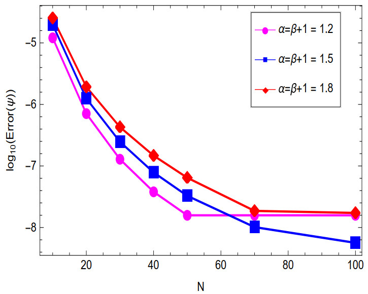
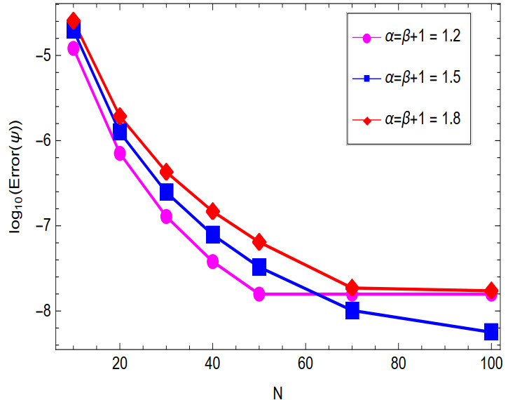
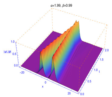
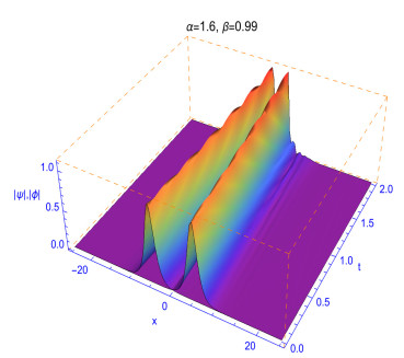
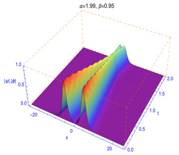
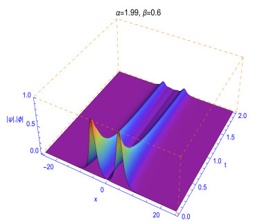
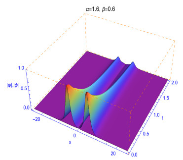
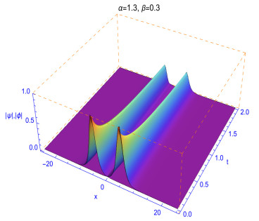
A coupled system of fractional order Gross-Pitaevskii equations is under consideration in which the time-fractional derivative is given in Caputo sense and the spatial fractional order derivative is of Riesz type. This kind of model may shed light on some time-evolution properties of the rotating two-component Bose¢ Einstein condensates. An unconditional convergent high-order scheme is proposed based on L2-$ 1_{\sigma} $ finite difference approximation in the time direction and Galerkin Legendre spectral approximation in the space direction. This combined scheme is designed in an easy algorithmic style. Based on ideas of discrete fractional Grönwall inequalities, we can prove the convergence theory of the scheme. Accordingly, a second order of convergence and a spectral convergence order in time and space, respectively, without any constraints on temporal meshes and the specified degree of Legendre polynomials $ N $. Some numerical experiments are proposed to support the theoretical results.
Citation: A.S. Hendy, R.H. De Staelen, A.A. Aldraiweesh, M.A. Zaky. High order approximation scheme for a fractional order coupled system describing the dynamics of rotating two-component Bose-Einstein condensates[J]. AIMS Mathematics, 2023, 8(10): 22766-22788. doi: 10.3934/math.20231160

Related Papers:

Abstract

A coupled system of fractional order Gross-Pitaevskii equations is under consideration in which the time-fractional derivative is given in Caputo sense and the spatial fractional order derivative is of Riesz type. This kind of model may shed light on some time-evolution properties of the rotating two-component Bose¢ Einstein condensates. An unconditional convergent high-order scheme is proposed based on L2-$ 1_{\sigma} $ finite difference approximation in the time direction and Galerkin Legendre spectral approximation in the space direction. This combined scheme is designed in an easy algorithmic style. Based on ideas of discrete fractional Grönwall inequalities, we can prove the convergence theory of the scheme. Accordingly, a second order of convergence and a spectral convergence order in time and space, respectively, without any constraints on temporal meshes and the specified degree of Legendre polynomials $ N $. Some numerical experiments are proposed to support the theoretical results.

References

[1]	M. Abbaszadeh, M. Dehghan, Y Zhou, Crank–nicolson/galerkin spectral method for solving two-dimensional time-space distributed-order weakly singular integro-partial differential equation, J. Comput. Appl. Math., 374 (2020), 112739.
[2]	M. Ainsworth, Z. Mao, Analysis and approximation of gradient flows associated with a fractional order gross–pitaevskii free energy, Commun. Appl. Math. Comput., 1 (2019), 5–19. https://doi.org/10.1007/s42967-019-0008-9 doi: 10.1007/s42967-019-0008-9
[3]	A. A. Alikhanov, A new difference scheme for the time fractional diffusion equation. J. Comput. Phys., 280 (2015), 424–438. https://doi.org/10.1016/j.jcp.2014.09.031 doi: 10.1016/j.jcp.2014.09.031
[4]	M. H. Anderson, J. R. Ensher, M. R. Matthews, C. E. Wieman, E. A. Cornell, Observation of Bose-Einstein condensation in a dilute atomic vapor, Science, 269 (1995), 198–201. https://doi.org/10.1126/science.269.5221.198 doi: 10.1126/science.269.5221.198
[5]	X. Antoine, W. Bao, C. Besse, Computational methods for the dynamics of the nonlinear schrödinger/gross–pitaevskii equations, Comput. Phys. Commun., 184 (2013), 2621–2633. https://doi.org/10.1016/j.cpc.2013.07.012 doi: 10.1016/j.cpc.2013.07.012
[6]	X. Antoine, R. Duboscq, Modeling and computation of bose-einstein condensates: Stationary states, nucleation, dynamics, stochasticity, Nonlinear Optical and Atomic Systems: at the Interface of Physics and Mathematics, 2015, 49–145. https://doi.org/10.1016/j.endm.2015.06.022 doi: 10.1016/j.endm.2015.06.022
[7]	X. Antoine, Q. Tang, J, Zhang, On the numerical solution and dynamical laws of nonlinear fractional schrödinger/gross–pitaevskii equations, Int. J. Comput. Math., 95 (2018), 1423–1443. https://doi.org/10.1080/00207160.2018.1437911 doi: 10.1080/00207160.2018.1437911
[8]	W. Bao, Y. Cai, Mathematical theory and numerical methods for bose-einstein condensation, Kinet. Relat. Mod., 6 (2013), 1.
[9]	B. Cheng, Z. Guo, D. Wang, Dissipativity of semilinear time fractional subdiffusion equations and numerical approximations, Appl. Math. Lett., 86 (2018), 276–283. https://doi.org/10.1016/j.aml.2018.07.006 doi: 10.1016/j.aml.2018.07.006
[10]	H. Ertik, H. Şirin, D. Demirhan, F. Büyükkiliç, Fractional mathematical investigation of Bose–Einstein condensation in dilute 87 Rb, 23 Na and 7 Li atomic gases, Int. J. Mod. Phys. B, 26 (2012), 1250096. https://doi.org/10.1142/S0217984912500960 doi: 10.1142/S0217984912500960
[11]	V. J. Ervin, J. P. Roop, Variational solution of fractional advection dispersion equations on bounded domains in $\mathbb{R}^d$, Numer. Meth. Part. D. E., 23 (2007), 256–281. https://doi.org/10.1002/num.20169 doi: 10.1002/num.20169
[12]	A. Griffin, D. W. Snoke, S. Stringari, Bose-einstein condensation. Cambridge University Press, 1996.
[13]	R. M. Hafez, M. A. Zaky, A. S. Hendy, A novel spectral Galerkin/Petrov–Galerkin algorithm for the multi-dimensional space–time fractional advection–diffusion–reaction equations with nonsmooth solutions, Math. Comput. Simulat., 190 (2021), 678–690. https://doi.org/10.1016/j.matcom.2021.06.004,2021 doi: 10.1016/j.matcom.2021.06.004,2021
[14]	A. S. Hendy, J. E. Macías-Díaz, A Conservative Scheme with Optimal Error Estimates for a Multidimensional Space–Fractional Gross–Pitaevskii Equation, Int. J. Appl. Math. Comput. Sci., 29 (2019), 713–723. https://doi.org/10.2478/amcs-2019-0053 doi: 10.2478/amcs-2019-0053
[15]	A. S. Hendy, J. E. Macías-Díaz, A discrete grönwall inequality and energy estimates in the analysis of a discrete model for a nonlinear time-fractional heat equation, Mathematics, 8 (2020), 1539.
[16]	A. S. Hendy, M. A. Zaky, Global consistency analysis of l1-galerkin spectral schemes for coupled nonlinear space-time fractional schrödinger equations, Appl. Numer. Math., 156 (2020), 276–302. https://doi.org/10.1016/j.apnum.2020.05.002 doi: 10.1016/j.apnum.2020.05.002
[17]	A. S. Hendy, M. A. Zaky, Graded mesh discretization for coupled system of nonlinear multi-term time-space fractional diffusion equations, Eng. Comput., 38 (2022), 1351–1363.
[18]	A. S. Hendy, M. A. Zaky, R. M. Hafez, R. H. De Staelen, The impact of memory effect on space fractional strong quantum couplers with tunable decay behavior and its numerical simulation, Sci. Rep., 2021, Article number: 10275. https://doi.org/10.1038/s41598-021-89701-7
[19]	P. Henning, A. Målqvist, The Finite Element Method for the Time-Dependent Gross–Pitaevskii Equation with Angular Momentum Rotation, SIAM J. Numer. Anal., 55 (2017), 923–952. https://doi.org/10.1137/15M1009172 doi: 10.1137/15M1009172
[20]	A. Jacob, P. G Juzeliūnas, L. Santos, Landau levels of cold atoms in non-Abelian gauge fields, New J. Phys., 10 (2008), 045022. https://doi.org/10.1088/1367-2630/10/4/045022 doi: 10.1088/1367-2630/10/4/045022
[21]	X. Li, L. Zhang, A conservative sine pseudo-spectral-difference method for multi-dimensional coupled Gross–Pitaevskii equations, Adv. Comput. Math., 46 (2020), 1–30.
[22]	X. Liang, A. Q. M. Khaliq, H. Bhatt, K. M. Furati, The locally extrapolated exponential splitting scheme for multi-dimensional nonlinear space-fractional schrödinger equations, Numer. Algorithms, 76 (2017), 939–958. https://doi.org/10.1007/s11075-017-0291-3 doi: 10.1007/s11075-017-0291-3
[23]	F. Liao, L. Zhang, Optimal error estimates of explicit finite difference schemes for the coupled Gross–Pitaevskii equations, Int. J. Comput. Math., 95 (2018), 1874–1892. https://doi.org/10.1080/00207160.2017.1343942 doi: 10.1080/00207160.2017.1343942
[24]	H. Liao, W. McLean, J. Zhang, A discrete Grönwall inequality with applications to numerical schemes for subdiffusion problems, SIAM J. Numer. Anal., 57 (2019), 218–237. https://doi.org/10.1137/16M1175742 doi: 10.1137/16M1175742
[25]	L. Pitaevskii, S. Stringari, Bose-Einstein condensation and superfluidity, 164 (2016), Oxford University Press.
[26]	I. Podlubny, Fractional Differential Equations. An Introduction to Fractional Derivatives, Fractional Differential Equations, Some Methods of Their Solution and Some of Their Applications, Mathematics in science and engineering; v. 198. Academic Press, San Diego, 1999.
[27]	A. Serna-Reyes, J. E. Macías-Díaz, A. Gallegos, N. Reguera, Cmmse: analysis and comparison of some numerical methods to solve a nonlinear fractional gross–pitaevskii system, J. Math. Chem., 60 (2022), 1272–1286. https://doi.org/10.1007/s10910-022-01360-9 doi: 10.1007/s10910-022-01360-9
[28]	J. Shen, Efficient spectral-galerkin method I. direct solvers of second-and fourth-order equations using legendre polynomials, SIAM J. Sci. Comput., 15 (1994), 1489–1505. https://doi.org/10.1137/0915089 doi: 10.1137/0915089
[29]	J. Shen, T. Tang, L. Wang, Spectral Methods: Algorithms, Analysis and Applications, 41 (2011), Springer Science & Business Media.
[30]	Z. Sun, D. Zhao, On the $L_\infty$ convergence of a difference scheme for coupled nonlinear Schrödinger equations, Comput. Math. Appl., 59 (2010), 3286–3300. https://doi.org/10.1016/j.camwa.2010.03.012 doi: 10.1016/j.camwa.2010.03.012
[31]	N. Uzar, S. Ballikaya, Investigation of classical and fractional Bose–Einstein condensation for harmonic potential, Physica A, 392 (2013), 1733–1741. https://doi.org/10.1016/j.physa.2012.11.039 doi: 10.1016/j.physa.2012.11.039
[32]	N. Uzar, D. Han, E. Aydiner, T. Tufekci, E. Aydıner, Solutions of the Gross-Pitaevskii and time-fractional Gross-Pitaevskii equations for different potentials with Homotopy Perturbation Method, arXiv preprint arXiv: 1203.3352, 2012.
[33]	T. Wang, Optimal point-wise error estimate of a compact difference scheme for the coupled Gross–Pitaevskii equations in one dimension, J. Sci. Comput., 59 (2014), 158–186. https://doi.org/10.1007/s10915-013-9757-1 doi: 10.1007/s10915-013-9757-1
[34]	Y. Wang, F. Liu, L. Mei, V. V. Anh, A novel alternating-direction implicit spectral galerkin method for a multi-term time-space fractional diffusion equation in three dimensions, Numer. Algorithms, 2020.
[35]	M. A. Zaky, A. S. Hendy, Convergence analysis of an L1-continuous Galerkin method for nonlinear time-space fractional Schrödinger equations, Int. J. Comput. Math., 98 (2021), 1420–1437. https://doi.org/10.1080/00207160.2020.1822994 doi: 10.1080/00207160.2020.1822994
[36]	M. A. Zaky, A. S. Hendy, J. E. Macías-Díaz, Semi-implicit galerkin–legendre spectral schemes for nonlinear time-space fractional diffusion–reaction equations with smooth and nonsmooth solutions, J. Sci. Comput., 82 (2020), Article number: 13.
[37]	F. Zeng, F. Liu, C. Li, K. Burrage, I. Turner, V. Anh, A crank–nicolson adi spectral method for a two-dimensional riesz space fractional nonlinear reaction-diffusion equation, SIAM J. Numer. Anal., 52 (2014), 2599–2622. https://doi.org/10.1137/130934192 doi: 10.1137/130934192
[38]	H. Zhang, X. Jiang, C. Wang, W. Fan, Galerkin-legendre spectral schemes for nonlinear space fractional schrödinger equation, Numer. Algorithms, 79 (2018), 337–356.
[39]	R. Zhang, Z. Han, Y. Shao, Z. Wang, Y. Wang, The numerical study for the ground and excited states of fractional bose–einstein condensates, Comput. Math. Appl., 78 (2019), 1548–1561.
[40]	Y. Zhang, W. Bao, H. Li, Dynamics of rotating two-component Bose–Einstein condensates and its efficient computation, Physica D., 234 (2007), 49–69. https://doi.org/10.1016/j.physd.2007.06.026 doi: 10.1016/j.physd.2007.06.026

Reader Comments

Your name:*

Email:*
© 2023 the Author(s), licensee AIMS Press. This is an open access article distributed under the terms of the Creative Commons Attribution License (http://creativecommons.org/licenses/by/4.0)