Vitamin D deficiency and Type 2 Diabetes (T2DM) are two important health problems that have rapidly increased prevalences in recent years. Chronic inflammation and susceptibility to infection are the characteristic features of T2DM. Vitamin D deficiency has been associated with high serum inflammatory marker levels due to its immunomodulatory effect. Moreover, studies have pointed out that vitamin D insufficiency could be associated with T2DM. Additionally, in recent years, inflammatory markers derived from hemogram have been associated with diabetes and its complications. Therefore, in our study, vitamin D levels, metabolic markers (i.e., serum uric acid, high-density lipoprotein (HDL) cholesterol, and low-density lipoprotein (LDL) cholesterol), and hemogram indices were analyzed in well controlled and poorly controlled T2DM patients. Furthermore, we compared those variables in vitamin D deficient and non-deficient groups.
Laboratory data, including vitamin D and hemogram markers, were compared between poorly and well controlled T2DM patients who visited the outpatient internal medicine clinics of our institution.
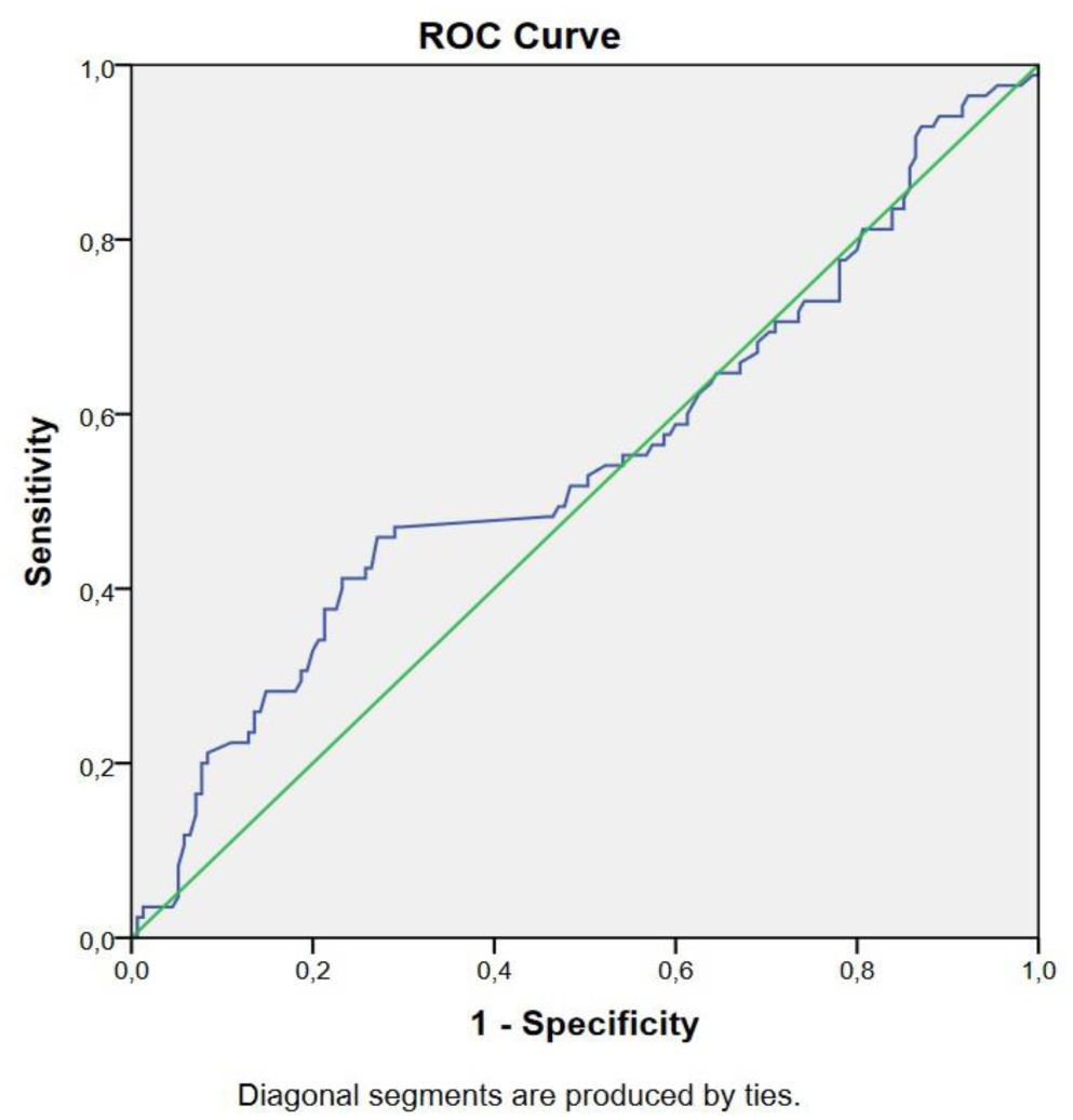
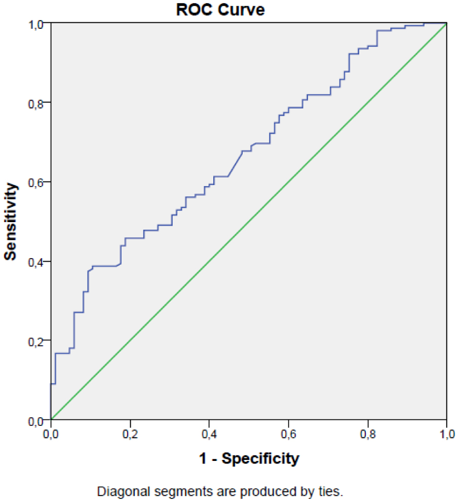
A total of 240 T2DM individuals were included in the present study: 170 individuals had vitamin D deficiency and 70 individuals had normal vitamin D levels, who served as controls. The median neutrophil to lymphocyte ratio (NLR) value was 2.2 (0.74–7.4) in the vitamin D deficient group and 2.02 (0.73–5.56) in the vitamin D normal group (p = 0.025). Among the study parameters, the NLR and glycated hemoglobin (HbA1c) levels showed a significant positive correlation (r = 0.30, p < 0.001). The sensitivity and specificity of the NLR to predict vitamin D deficiency were determined as 60% and 49%, respectively (AUC: 0.59, p = 0.03, 95% CI: 0.51–0.67). The sensitivity and specificity of the NLR to predict an improved control of diabetes were 72% and 45%, respectively (AUC: 0.67, p < 0.001, 95% CI: 0.60–0.74).
We think that NLR can be helpful in follow up of T2DM and vitamin D deficiency.
Citation: Elif Basaran, Gulali Aktas. The relationship of vitamin D levels with hemogram indices and metabolic parameters in patients with type 2 diabetes mellitus[J]. AIMS Medical Science, 2024, 11(1): 47-57. doi: 10.3934/medsci.2024004
Vitamin D deficiency and Type 2 Diabetes (T2DM) are two important health problems that have rapidly increased prevalences in recent years. Chronic inflammation and susceptibility to infection are the characteristic features of T2DM. Vitamin D deficiency has been associated with high serum inflammatory marker levels due to its immunomodulatory effect. Moreover, studies have pointed out that vitamin D insufficiency could be associated with T2DM. Additionally, in recent years, inflammatory markers derived from hemogram have been associated with diabetes and its complications. Therefore, in our study, vitamin D levels, metabolic markers (i.e., serum uric acid, high-density lipoprotein (HDL) cholesterol, and low-density lipoprotein (LDL) cholesterol), and hemogram indices were analyzed in well controlled and poorly controlled T2DM patients. Furthermore, we compared those variables in vitamin D deficient and non-deficient groups.
Laboratory data, including vitamin D and hemogram markers, were compared between poorly and well controlled T2DM patients who visited the outpatient internal medicine clinics of our institution.
A total of 240 T2DM individuals were included in the present study: 170 individuals had vitamin D deficiency and 70 individuals had normal vitamin D levels, who served as controls. The median neutrophil to lymphocyte ratio (NLR) value was 2.2 (0.74–7.4) in the vitamin D deficient group and 2.02 (0.73–5.56) in the vitamin D normal group (p = 0.025). Among the study parameters, the NLR and glycated hemoglobin (HbA1c) levels showed a significant positive correlation (r = 0.30, p < 0.001). The sensitivity and specificity of the NLR to predict vitamin D deficiency were determined as 60% and 49%, respectively (AUC: 0.59, p = 0.03, 95% CI: 0.51–0.67). The sensitivity and specificity of the NLR to predict an improved control of diabetes were 72% and 45%, respectively (AUC: 0.67, p < 0.001, 95% CI: 0.60–0.74).
We think that NLR can be helpful in follow up of T2DM and vitamin D deficiency.

| [1] | Rudnicka E, Suchta K, Grymowicz M, et al. (2021) Chronic Low Grade Inflammation in Pathogenesis of PCOS. Int J Mol Sci 22. https://doi.org/10.3390/ijms22073789 |
| [2] |
Salvatore T, Carbonara O, Cozzolino D, et al. (2009) Progress in the oral treatment of type 2 diabetes: update on DPP-IV inhibitors. Curr Diab Rep 5: 92-101. https://doi.org/10.2174/157339909788166819 
|
| [3] |
Petersmann A, Müller-Wieland D, Müller UA, et al. (2019) Definition, Classification and Diagnosis of Diabetes Mellitus. Exp Clin Endocrinol Diabetes 127: S1-S7. https://doi.org/10.1055/a-1018-9078
|
| [4] |
Cloete L (2022) Diabetes mellitus: an overview of the types, symptoms, complications and management. Nursing Standard 37: 61-66. https://doi.org/10.7748/ns.2021.e11709
|
| [5] |
Erkus E, Aktas G, Kocak MZ, et al. (2019) Diabetic regulation of subjects with type 2 diabetes mellitus is associated with serum vitamin D levels. Rev Assoc Med Bras 65: 51-55. https://doi.org/10.1590/1806-9282.65.1.51
|
| [6] |
Argano C, Mirarchi L, Amodeo S, et al. (2023) The Role of Vitamin D and Its Molecular Bases in Insulin Resistance, Diabetes, Metabolic Syndrome, and Cardiovascular Disease: State of the Art. Int J Mol Sci 24: 15485. https://doi.org/10.3390/ijms242015485
|
| [7] |
Berridge MJ (2017) Vitamin D deficiency and diabetes. Biochem J 474: 1321-1332. https://doi.org/10.1042/bcj20170042
|
| [8] |
Sacerdote A, Dave P, Lokshin V, et al. (2019) Type 2 Diabetes Mellitus, Insulin Resistance, and Vitamin D. Curr Diab Rep 19: 101. https://doi.org/10.1007/s11892-019-1201-y
|
| [9] |
Ceriello A, Prattichizzo F (2021) Variability of risk factors and diabetes complications. Cardiovasc Diabetol 20: 101. https://doi.org/10.1186/s12933-021-01289-4
|
| [10] |
Mitri J, Pittas AG (2014) Vitamin D and diabetes. Endocrin Metab Clin 43: 205-232. https://doi.org/10.1016/j.ecl.2013.09.010
|
| [11] |
Forsythe LK, Livingstone MB, Barnes MS, et al. (2012) Effect of adiposity on vitamin D status and the 25-hydroxycholecalciferol response to supplementation in healthy young and older Irish adults. Br J Nutr 107: 126-134. https://doi.org/10.1017/s0007114511002662
|
| [12] |
Bener A, Al-Hamaq AO, Kurtulus EM, et al. (2016) The role of vitamin D, obesity and physical exercise in regulation of glycemia in Type 2 Diabetes Mellitus patients. Diabetes Metab Syndr 10: 198-204. https://doi.org/10.1016/j.dsx.2016.06.007
|
| [13] | Erkus E, Aktas G, Atak BM, et al. (2018) Haemogram Parameters in Vitamin D Deficiency. J Coll Physicians Surg Pak 28: 779-782. |
| [14] |
Aspell N, Laird E, Healy M, et al. (2019) Vitamin D Deficiency Is Associated With Impaired Muscle Strength And Physical Performance In Community-Dwelling Older Adults: Findings From The English Longitudinal Study Of Ageing. Clin Interv Aging 14: 1751-1761. https://doi.org/10.2147/CIA.S222143
|
| [15] |
Remelli F, Vitali A, Zurlo A, et al. (2019) Vitamin D Deficiency and Sarcopenia in Older Persons. Nutrients 11: 2861. https://doi.org/10.3390/nu11122861
|
| [16] |
Afzal S, Bojesen SE, Nordestgaard BG (2013) Low 25-hydroxyvitamin D and risk of type 2 diabetes: a prospective cohort study and metaanalysis. Clin Chem 59: 381-391. https://doi.org/10.1373/clinchem.2012.193003
|
| [17] |
Chiu KC, Chuang LM, Yoon C (2001) The vitamin D receptor polymorphism in the translation initiation codon is a risk factor for insulin resistance in glucose tolerant Caucasians. BMC Med Genet 2: 2. https://doi.org/10.1186/1471-2350-2-2
|
| [18] |
Forouhi NG, Ye Z, Rickard AP, et al. (2012) Circulating 25-hydroxyvitamin D concentration and the risk of type 2 diabetes: results from the European Prospective Investigation into Cancer (EPIC)-Norfolk cohort and updated meta-analysis of prospective studies. Diabetologia 55: 2173-2182. https://doi.org/10.1007/s00125-012-2544-y
|
| [19] |
Meddeb N, Sahli H, Chahed M, et al. (2005) Vitamin D deficiency in Tunisia. Osteoporos Int 16: 180-183. https://doi.org/10.1007/s00198-004-1658-6
|
| [20] |
Lips P, Cashman KD, Lamberg-Allardt C, et al. (2019) Current vitamin D status in European and Middle East countries and strategies to prevent vitamin D deficiency: a position statement of the European Calcified Tissue. Society Eur. J Endocrinol 180: P23-p54. https://doi.org/10.1530/eje-18-0736
|
| [21] |
Baker MR, Peacock M, Nordin BE (1980) The decline in vitamin D status with age. Age Ageing 9: 249-252. https://doi.org/10.1093/ageing/9.4.249
|
| [22] |
Liu E, Meigs JB, Pittas AG, et al. (2010) Predicted 25-hydroxyvitamin D score and incident type 2 diabetes in the Framingham Offspring Study. Am J Clin Nutr 91: 1627-1633. https://doi.org/10.3945/ajcn.2009.28441
|
| [23] |
Targher G, Bertolini L, Padovani R, et al. (2006) Serum 25-hydroxyvitamin D3 concentrations and carotid artery intima-media thickness among type 2 diabetic patients. Clin Endocrinol 65: 593-597. https://doi.org/10.1111/j.1365-2265.2006.02633.x
|
| [24] |
Wang Y, Si S, Liu J, et al. (2016) The Associations of Serum Lipids with Vitamin D Status. PloS One 11: e0165157. https://doi.org/10.1371/journal.pone.0165157
|
| [25] |
Goldberg IJ (2001) Clinical review 124: Diabetic dyslipidemia: causes and consequences. J Clin Endocrinol Metab 86: 965-971. https://doi.org/10.1210/jcem.86.3.7304
|
| [26] |
Zhao Y, Yin L, Patel J, et al. (2021) The inflammatory markers of multisystem inflammatory syndrome in children (MIS-C) and adolescents associated with COVID-19: A meta-analysis. J Med Virol 93: 4358-4369. https://doi.org/10.1002/jmv.26951
|
| [27] |
Cigolini M, Iagulli MP, Miconi V, et al. (2006) Serum 25-hydroxyvitamin D3 concentrations and prevalence of cardiovascular disease among type 2 diabetic patients. Diabetes Care 29: 722-724. https://doi.org/10.2337/diacare.29.03.06.dc05-2148
|
| [28] |
Chen N, Wan Z, Han SF, et al. (2014) Effect of vitamin D supplementation on the level of circulating high-sensitivity C-reactive protein: a meta-analysis of randomized controlled trials. Nutrients 6: 2206-2216. https://doi.org/10.3390/nu6062206
|
| [29] | Skolmowska D, Głąbska D, Kołota A, et al. (2022) Effectiveness of Dietary Interventions to Treat Iron-Deficiency Anemia in Women: A Systematic Review of Randomized Controlled Trials. Nutrients 14. https://doi.org/10.3390/nu14132724 |
| [30] |
Aktas G, Duman TT, Atak B, et al. (2020) Irritable bowel syndrome is associated with novel inflammatory markers derived from hemogram parameters. Fam Med Prim Care Rev 22: 107-110. https://doi.org/10.5114/fmpcr.2020.95311
|
Figures(2) / Tables(4)

Elif Basaran, Gulali Aktas. The relationship of vitamin D levels with hemogram indices and metabolic parameters in patients with type 2 diabetes mellitus[J]. AIMS Medical Science, 2024, 11(1): 47-57. doi: 10.3934/medsci.2024004


 DownLoad: