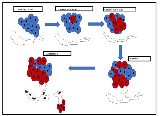
Cancer is a disease that arises from the uncontrolled growth of abnormal (tumor) cells in an organ and their subsequent spread into other parts of the body. If tumor cells spread to surrounding tissues or other organs, then the disease is life-threatening due to limited treatment options. This work applies an agent-based model to investigate the effect of intra-tumoral communication on tumor progression, plasticity, and invasion, with results suggesting that cell-cell and cell-extracellular matrix (ECM) interactions affect tumor cell behavior. Additionally, the model suggests that low initial healthy cell densities and ECM protein densities promote tumor progression, cell motility, and invasion. Furthermore, high ECM breakdown probabilities of tumor cells promote tumor invasion. Understanding the intra-tumoral communication under cellular stress can potentially lead to the design of successful treatment strategies for cancer.
Citation: Hasitha N. Weerasinghe, Pamela M. Burrage, Dan V. Nicolau Jr., Kevin Burrage. Agent-based modeling for the tumor microenvironment (TME)[J]. Mathematical Biosciences and Engineering, 2024, 21(11): 7621-7647. doi: 10.3934/mbe.2024335
Cancer is a disease that arises from the uncontrolled growth of abnormal (tumor) cells in an organ and their subsequent spread into other parts of the body. If tumor cells spread to surrounding tissues or other organs, then the disease is life-threatening due to limited treatment options. This work applies an agent-based model to investigate the effect of intra-tumoral communication on tumor progression, plasticity, and invasion, with results suggesting that cell-cell and cell-extracellular matrix (ECM) interactions affect tumor cell behavior. Additionally, the model suggests that low initial healthy cell densities and ECM protein densities promote tumor progression, cell motility, and invasion. Furthermore, high ECM breakdown probabilities of tumor cells promote tumor invasion. Understanding the intra-tumoral communication under cellular stress can potentially lead to the design of successful treatment strategies for cancer.

| [1] |
R. Baghban, L. Roshangar, R. Jahanban-Esfahlan, K. Seidi, A. Ebrahimi-Kalan, M. Jaymand, et al., Tumor microenvironment complexity and therapeutic implications at a glance, Cell Commun. Signaling, 18 (2020), 1–19. https://doi.org/10.1186/s12964-020-0530-4 doi: 10.1186/s12964-020-0530-4

|
| [2] |
F. R. Balkwill, M. Capasso, T. Hagemann, The tumor microenvironment at a glance, J. Cell Sci., 125 (2012), 5591–5596. https://doi.org/10.1242/jcs.116392 doi: 10.1242/jcs.116392
|
| [3] |
B. Coban, C. Bergonzini, A. J. Zweemer, E. H. Danen, Metastasis: crosstalk between tissue mechanics and tumour cell plasticity, Br. J. Cancer, 124 (2021), 49–57. https://doi.org/10.1038/s41416-020-01150-7 doi: 10.1038/s41416-020-01150-7
|
| [4] |
M. L. Taddei, E. Giannoni, G. Comito, P. Chiarugi, Microenvironment and tumor cell plasticity: an easy way out, Cancer Lett., 341 (2013), 80–96. https://doi.org/10.1016/j.canlet.2013.01.042 doi: 10.1016/j.canlet.2013.01.042
|
| [5] |
A. L. Ribeiro, O. K. Okamoto, Combined effects of pericytes in the tumor microenvironment, Stem Cells Int., 1 (2015), 868475. https://doi.org/10.1155/2015/868475 doi: 10.1155/2015/868475
|
| [6] | B. M. Lopes-Bastos, W. G. Jiang, J. Cai, Tumour-endothelial cell communications: important and indispensable mediators of tumour angiogenesis, Anticancer Res., 36 (2016), 1119–1126. |
| [7] |
F. Xing, J. Saidou, K. Watabe, Cancer associated fibroblasts (CAFs) in tumor microenvironment, Front. Biosci., 15 (2010), 166. https://doi.org/10.2741/3613 doi: 10.2741/3613
|
| [8] |
M. R. Galdiero, E. Bonavita, I. Barajon, C. Garlanda, A. Mantovani, S. Jaillon, Tumor associated macrophages and neutrophils in cancer, Immunobiology, 218 (2013), 1402–1410. https://doi.org/10.1016/j.imbio.2013.06.003 doi: 10.1016/j.imbio.2013.06.003
|
| [9] |
A. M. Høye, J. T. Erler, Structural ECM components in the premetastatic and metastatic niche, Am. J. Physiol. Cell Physiol., 310 (2016), C955–C967. https://doi.org/10.1152/ajpcell.00326.2015 doi: 10.1152/ajpcell.00326.2015
|
| [10] |
P. Lu, V. M. Weaver, Z. Werb, The extracellular matrix: a dynamic niche in cancer progression, J. Cell Biol., 196 (2012), 395–406. https://doi.org/10.1083/jcb.201102147 doi: 10.1083/jcb.201102147
|
| [11] |
A. D. Theocharis, S. S. Skandalis, C. Gialeli, N. K. Karamanos, Extracellular matrix structure, Adv. Drug Delivery Rev., 97 (2016), 4–27. https://doi.org/10.1016/j.addr.2015.11.001 doi: 10.1016/j.addr.2015.11.001
|
| [12] |
B. Yue, Biology of the extracellular matrix: an overview, J. Glaucoma, 23 (2014), S20–S23. https://doi.org/10.1097/IJG.0000000000000108 doi: 10.1097/IJG.0000000000000108
|
| [13] |
J. Huang, L. Zhang, D. Wan, L. Zhou, S. Zheng, S. Lin, et al., Extracellular matrix and its therapeutic potential for cancer treatment, Signal Transduction Targeted Ther., 6 (2021), 1–24. https://doi.org/10.1038/s41392-021-00544-0 doi: 10.1038/s41392-021-00544-0
|
| [14] | K. Yuan, R. K. Singh, G. Rezonzew, G. P. Siegal, In vitro matrices for studying tumor cell invasion, in Cell Motility in Cancer Invasion and Metastasis, Springer, (2006), 25–54. https://doi.org/10.1007/b103440 |
| [15] |
N. M. Hooper, Y. Itoh, H. Nagase, Matrix metalloproteinases in cancer, Essays Biochem., 38 (2002), 21–36. https://doi.org/10.1042/bse0380021 doi: 10.1042/bse0380021
|
| [16] |
L. A. Liotta, U. P. Thorgeirsson, S. Garbisa, Role of collagenases in tumor cell invasion, Cancer Metastasis Rev., 1 (1982), 277–288. https://doi.org/10.1007/BF00124213 doi: 10.1007/BF00124213
|
| [17] | T. R. Cox, The matrix in cancer, Nat. Rev. Cancer, 21 (2021), 217–238. https://doi.org/10.1038/s41568-020-00329-7 |
| [18] |
S. Turner, J. A. Sherratt, Intercellular adhesion and cancer invasion: a discrete simulation using the extended potts model, J. Theor. Biol., 216 (2002), 85–100. https://doi.org/10.1006/jtbi.2001.2522 doi: 10.1006/jtbi.2001.2522
|
| [19] |
M. DePalma, D. Biziato, T. V. Petrova, Microenvironmental regulation of tumour angiogenesis, Nat. Rev. Cancer, 17 (2017), 457–474. https://doi.org/10.1038/nrc.2017.51 doi: 10.1038/nrc.2017.51
|
| [20] |
R. J. Gillies, J. S. Brown, A. R. Anderson, R. A. Gatenby, Eco-evolutionary causes and consequences of temporal changes in intratumoural blood flow, Nat. Rev. Cancer, 18 (2018), 576–585. https://doi.org/10.1038/s41568-018-0030-7 doi: 10.1038/s41568-018-0030-7
|
| [21] |
B. T. Finicle, V. Jayashankar, A. L. Edinger, Nutrient scavenging in cancer, Nat. Rev. Cancer, 18 (2018), 619–633. https://doi.org/10.1038/s41568-018-0048-x doi: 10.1038/s41568-018-0048-x
|
| [22] | C. García-Jiménez, C. R. Goding, Starvation and pseudo-starvation as drivers of cancer metastasis through translation reprogramming, Cell Metab., 29 (2019), 254–267. |
| [23] |
R. J. DeBerardinis, N. S. Chandel, Fundamentals of cancer metabolism, Sci. Adv., 2 (2016), e1600200. https://doi.org/10.1126/sciadv.1600200 doi: 10.1126/sciadv.1600200
|
| [24] |
M. G. Vander Heiden, Targeting cancer metabolism: a therapeutic window opens, Nat. Rev. Drug Discovery, 10 (2011), 671–684. https://doi.org/10.1038/nrd3504 doi: 10.1038/nrd3504
|
| [25] |
B. Kalyanaraman, Teaching the basics of cancer metabolism: Developing antitumor strategies by exploiting the differences between normal and cancer cell metabolism, Redox Biol., 12 (2017), 833–842. https://doi.org/10.1016/j.redox.2017.04.018 doi: 10.1016/j.redox.2017.04.018
|
| [26] |
R. A. Cairns, I. S. Harris, T. W. Mak, Regulation of cancer cell metabolism, Nat. Rev. Cancer, 11 (2011), 85–95. https://doi.org/10.1038/nrc2981 doi: 10.1038/nrc2981
|
| [27] |
C. A. Lyssiotis, A. C. Kimmelman, Metabolic interactions in the tumor microenvironment, Trends Cell Biol., 27 (2017), 863–875. https://doi.org/10.1016/j.tcb.2017.06.003 doi: 10.1016/j.tcb.2017.06.003
|
| [28] |
S. Bowling, K. Lawlor, T. A. Rodríguez, Cell competition: the winners and losers of fitness selection, Development, 146 (2019), dev167486. https://doi.org/10.1242/dev.167486 doi: 10.1242/dev.167486
|
| [29] |
A. Gutiérrez-Martínez, W. Q. G. Sew, M. Molano-Fernández, M. Carretero-Junquera, H. Herranz, Mechanisms of oncogenic cell competition-paths of victory, Semin. Cancer Biol., 63 (2020), 27–35. https://doi.org/10.1016/j.semcancer.2019.05.015 doi: 10.1016/j.semcancer.2019.05.015
|
| [30] |
R. Levayer, Solid stress, competition for space and cancer: The opposing roles of mechanical cell competition in tumour initiation and growth, Nat. Rev. Cancer, 63 (2020), 69–80. https://doi.org/10.1016/j.semcancer.2019.05.004 doi: 10.1016/j.semcancer.2019.05.004
|
| [31] |
E. Moreno, Is cell competition relevant to cancer?, Nat. Rev. Cancer, 8 (2008), 141–147. https://doi.org/10.1038/nrc2252 doi: 10.1038/nrc2252
|
| [32] | M. Vishwakarma, E. Piddini, Outcompeting cancer, Nat. Rev. Cancer, 20 (2020), 187–198. https://doi.org/10.1038/s41568-019-0231-8 |
| [33] |
T. M. Parker, V. Henriques, A. Beltran, H. Nakshatri, R. Gogna, Cell competition and tumor heterogeneity, Nat. Rev. Cancer, 63 (2020), 1–10. https://doi.org/10.1016/j.semcancer.2019.09.003 doi: 10.1016/j.semcancer.2019.09.003
|
| [34] |
S. Di Giacomo, M. Sollazzo, D. De Biase, M. Ragazzi, P. Bellosta, A. Pession, et al., Human cancer cells signal their competitive fitness through MYC activity, Sci. Rep., 7 (2017), 1–12. https://doi.org/10.1038/s41598-017-13002-1 doi: 10.1038/s41598-017-13002-1
|
| [35] |
E. Madan, M. L. Peixoto, P. Dimitrion, T. D. Eubank, M. Yekelchyk, S. Talukdar, et al., Cell competition boosts clonal evolution and hypoxic selection in cancer, Trends Cell Biol., 12 (2020), 967–978. https://doi.org/10.1016/j.tcb.2020.10.002 doi: 10.1016/j.tcb.2020.10.002
|
| [36] |
U. Cavallaro, G. Christofori, Cell adhesion in tumor invasion and metastasis: loss of the glue is not enough, Biochim. Biophys. Acta, Rev. Cancer, 1552 (2001), 39–45. https://doi.org/10.1016/S0304-419X(01)00038-5 doi: 10.1016/S0304-419X(01)00038-5
|
| [37] |
M. Janiszewska, M. C. Primi, T. Izard, Cell adhesion in cancer: Beyond the migration of single cells, J. Biol. Chem., 295 (2020), 2495–2505. https://doi.org/10.1074/jbc.REV119.007759 doi: 10.1074/jbc.REV119.007759
|
| [38] |
M. C. Moh, S. Shen, The roles of cell adhesion molecules in tumor suppression and cell migration: a new paradox, Cell Adhes. Migr., 3 (2009), 334–336. https://doi.org/10.4161/cam.3.4.9246 doi: 10.4161/cam.3.4.9246
|
| [39] |
H. Son, A. Moon, Epithelial-mesenchymal transition and cell invasion, Toxicol. Res., 26 (2010), 245–252. https://doi.org/10.5487/TR.2010.26.4.245 doi: 10.5487/TR.2010.26.4.245
|
| [40] |
P. M. Altrock, L. L. Liu, F. Michor, The mathematics of cancer: integrating quantitative models, Nat. Rev. Cancer, 15 (2015), 730–745. https://doi.org/10.1038/nrc4029 doi: 10.1038/nrc4029
|
| [41] |
G. Jordão, J. N. Tavares, Mathematical models in cancer therapy, Biosystems, 162 (2017), 12–23. https://doi.org/10.1016/j.biosystems.2017.08.007 doi: 10.1016/j.biosystems.2017.08.007
|
| [42] |
V. Quaranta, A. M. Weaver, P. T. Cummings, A. R. Anderson, Mathematical modeling of cancer: The future of prognosis and treatment, Clin. Chim. Acta, 357 (2005), 173–179. https://doi.org/10.1016/j.cccn.2005.03.023 doi: 10.1016/j.cccn.2005.03.023
|
| [43] |
H. N. Weerasinghe, P. M. Burrage, K. Burrage, D. V. Nicolau Jr, Mathematical models of cancer cell plasticity, J. Oncol., 2019 (2019), 2403483. https://doi.org/10.1155/2019/2403483 doi: 10.1155/2019/2403483
|
| [44] | P. Macklin, M. E. Edgerton, Discrete cell modeling, in Multiscale Modeling of Cancer: an Integrated Experimental and Mathematical Modeling Approach, Cambridge University Press, (2010), 88–122. https://doi.org/10.1017/CBO9780511781452 |
| [45] |
J. Metzcar, Y. Wang, R. Heiland, P. Macklin, A review of cell-based computational modeling in cancer biology, JCO Clin. Cancer Inf., 2 (2019), 1–13. https://doi.org/10.1200/CCI.18.00069 doi: 10.1200/CCI.18.00069
|
| [46] |
Z. Wang, J. D. Butner, V. Cristini, T. S. Deisboeck, Integrated PK-PD and agent-based modeling in oncology, J. Pharmacokinet. Pharmacodyn., 42 (2015), 179189. https://doi.org/10.1007/s10928-015-9403-7 doi: 10.1007/s10928-015-9403-7
|
| [47] |
C. K. Macnamara, Biomechanical modelling of cancer: Agent-based force-based models of solid tumours within the context of the tumour microenvironment, Comput. Syst. Oncol., 1 (2021), e1018. https://doi.org/10.1002/cso2.1018 doi: 10.1002/cso2.1018
|
| [48] |
J. S. Lowengrub, H. B. Frieboes, F. Jin, Y. L. Chuang, X. Li, P. Macklin, et al., Nonlinear modelling of cancer: bridging the gap between cells and tumours, Nonlinearity, 23 (2009), R1–R91. https://doi.org/10.1088/0951-7715/23/1/R01 doi: 10.1088/0951-7715/23/1/R01
|
| [49] |
R. Sachs, L. Hlatky, P. Hahnfeldt, Simple ODE models of tumor growth and anti-angiogenic or radiation treatment, Math. Comput. Modell., 33 (2001), 1297–1305. https://doi.org/10.1016/S0895-7177(00)00316-2 doi: 10.1016/S0895-7177(00)00316-2
|
| [50] |
H. Enderling, A. R. Anderson, M. A. Chaplain, A. J. Munro, J. S. Vaidya, Mathematical modelling of radiotherapy strategies for early breast cancer, J. Theor. Biol., 241 (2006), 158–171. https://doi.org/10.1016/j.jtbi.2005.11.015 doi: 10.1016/j.jtbi.2005.11.015
|
| [51] | H. Enderling, M. A. Chaplain, A. R. Anderson, J. S. Vaidya, A mathematical model of breast cancer development, local treatment and recurrence, J. Theor. Biol., 246 (2007), 245–259. |
| [52] |
V. Andasari, M. A. Chaplain, Intracellular modelling of cell-matrix adhesion during cancer cell invasion, Math. Modell. Nat. Phenom., 7 (2012), 29–48. https://doi.org/10.1051/mmnp/20127103 doi: 10.1051/mmnp/20127103
|
| [53] | J. C. Larsen, A mathematical model of adoptive T cell therapy, JP J. Appl. Math., 15 (2017), 1–33. |
| [54] |
L. Glass, Instability and mitotic patterns in tissue growth, IFAC Proc. Vol., 6 (1973), 129–131. https://doi.org/10.1016/S1474-6670(17)67989-8 doi: 10.1016/S1474-6670(17)67989-8
|
| [55] |
R. Shymko, L. Glass, Cellular and geometric control of tissue growth and mitotic instability, J. Theor. Biol., 63 (1976), 355–374. https://doi.org/10.1016/0022-5193(76)90039-4 doi: 10.1016/0022-5193(76)90039-4
|
| [56] |
M. Chaplain, Avascular growth, angiogenesis and vascular growth in solid tumours: The mathematical modelling of the stages of tumour development, Math. Comput. Modell., 23 (1996), 47–87. https://doi.org/10.1016/0895-7177(96)00019-2 doi: 10.1016/0895-7177(96)00019-2
|
| [57] |
J. A. Adam, A simplified mathematical model of tumor growth, Math. Biosci., 81 (1986), 229–244. https://doi.org/10.1016/0025-5564(86)90119-7 doi: 10.1016/0025-5564(86)90119-7
|
| [58] |
J. A. Adam, A mathematical model of tumor growth by diffusion, Math. Biosci., 94 (1989), 155. https://doi.org/10.1016/0895-7177(88)90533-X doi: 10.1016/0895-7177(88)90533-X
|
| [59] |
J. A. Adam, S. Maggelakis, Mathematical models of tumor growth. iv. effects of a necrotic core, Math. Biosci., 97 (1989), 121–136. https://doi.org/10.1016/0025-5564(89)90045-X doi: 10.1016/0025-5564(89)90045-X
|
| [60] | T. S. Deisboeck, Z. Wang, P. Macklin, V. Cristini, Multiscale cancer modeling, Ann. Rev. Biomed. Eng., 13 (2011), 127–155. https://doi.org/10.1201/b10407 |
| [61] | E. Gavagnin, C. A. Yates, Stochastic and deterministic modeling of cell migration, in Handbook of Statistics, 39 (2018), 37–91. https://doi.org/10.1016/bs.host.2018.06.002 |
| [62] |
A. S. Qi, X. Zheng, C. Y. Du, B. S. An, A cellular automaton model of cancerous growth, J. Theor. Biol., 161 (1993), 1–12. https://doi.org/10.1006/jtbi.1993.1035 doi: 10.1006/jtbi.1993.1035
|
| [63] |
J. Smolle, R. Hofmann-Wellenhof, R. Kofler, L. Cerroni, J. Haas, H. Kerl, Computer simulations of histologic patterns in melanoma using a cellular automaton provide correlations with prognosis, J. Invest. Dermatol., 105 (1995), 797–801. https://doi.org/10.1111/1523-1747.ep12326559 doi: 10.1111/1523-1747.ep12326559
|
| [64] |
S. F. Junior, M. Martins, M. Vilela, A growth model for primary cancer, Physica A, 261 (1998), 569–580. https://doi.org/10.1016/S0378-4371(98)00318-5 doi: 10.1016/S0378-4371(98)00318-5
|
| [65] |
H. Hatzikirou, A. Deutsch, Cellular automata as microscopic models of cell migration in heterogeneous environments, Curr. Topics Dev. Biol., 81 (2008), 401–434. https://doi.org/10.1016/S0070-2153(07)81014-3 doi: 10.1016/S0070-2153(07)81014-3
|
| [66] |
B. Chopard, R. Ouared, A. Deutsch, H. Hatzikirou, D. Wolf-Gladrow, Lattice-gas cellular automaton models for biology: from fluids to cells, Acta Biotheor., 58 (2010), 329–340. https://doi.org/10.1007/s10441-010-9118-5 doi: 10.1007/s10441-010-9118-5
|
| [67] |
Y. Jiang, J. Pjesivac-Grbovic, C. Cantrell, J. P. Freyer, A multiscale model for avascular tumor growth, Biophys. J., 89 (2005), 3884–3894. https://doi.org/10.1529/biophysj.105.060640 doi: 10.1529/biophysj.105.060640
|
| [68] |
A. Shirinifard, J. S. Gens, B. L. Zaitlen, N. J. Popławski, M. Swat, J. A. Glazier, 3D multi-cell simulation of tumor growth and angiogenesis, PloS One, 4 (2009), e7190. https://doi.org/10.1371/journal.pone.0007190 doi: 10.1371/journal.pone.0007190
|
| [69] |
A. Szabó, R. M. Merks, Cellular potts modeling of tumor growth, tumor invasion, and tumor evolution, Front. Oncol., 3 (2013), 87. https://doi.org/10.3389/fonc.2013.00087 doi: 10.3389/fonc.2013.00087
|
| [70] |
C. E. Donaghey, CELLSIM: cell cycle simulation made easy, Int. Rev. Cytol., 66 (1980), 171–210. https://doi.org/10.1016/S0074-7696(08)61974-9 doi: 10.1016/S0074-7696(08)61974-9
|
| [71] |
W. Duchting, G. Dehl, Spatial structure of tumor growth: A simulation study, IEEE Trans. Syst. Man Cybern., 10 (1980), 292–296. https://doi.org/10.1109/TSMC.1980.4308502 doi: 10.1109/TSMC.1980.4308502
|
| [72] |
W. Duchting, T. Vogelsaenger, Aspects of modelling and simulating tumor growth and treatment, J. Cancer Res. Clin. Oncol., 105 (1983), 1–12. https://doi.org/10.1007/BF00391824 doi: 10.1007/BF00391824
|
| [73] |
W. Duchting, T. Vogelsaenger, Recent progress in modelling and simulation of three dimensional tumor growth and treatment, Biosystems, 18 (1985), 79–91. https://doi.org/10.1016/0303-2647(85)90061-9 doi: 10.1016/0303-2647(85)90061-9
|
| [74] |
W. Duchting, T. Vogelsaenger, Three-dimensional pattern generation applied to spheroidal tumor growth in a nutrient medium, Int. J. Biomed. Comput., 12 (1981), 377–392. https://doi.org/10.1016/0020-7101(81)90050-7 doi: 10.1016/0020-7101(81)90050-7
|
| [75] | W. Duchting, T. Ginsberg, W. Ulmer, Modelling of tumor growth and treatment, Z. Angew. Math. Mech., 76 (1996), 347–350. |
| [76] |
J. E. Schmitz, A. R. Kansaland, S. Torquato, A cellular automaton model of brain tumor treatment and resistance, J. Theor. Med., 4 (2002), 223–239. https://doi.org/10.1080/1027366031000086674 doi: 10.1080/1027366031000086674
|
| [77] |
C. Gong, O. Milberg, B. Wang, P. Vicini, R. Narwal, L. Roskos, et al., A computational multiscale agent-based model for simulating spatio-temporal tumour immune response to PD1 and PDL1 inhibition, J. R. Soc. Interface, 14 (2017), 20170320. https://doi.org/10.1098/rsif.2017.0320 doi: 10.1098/rsif.2017.0320
|
| [78] |
H. Xie, Y. Jiao, Q. Fan, M. Hai, J. Yang, Z. Hu, et al., Modeling three-dimensional invasive solid tumor growth in heterogeneous microenvironment under chemotherapy, PloS One, 13 (2018), e0206292. https://doi.org/10.1371/journal.pone.0206292 doi: 10.1371/journal.pone.0206292
|
| [79] |
A. R. Anderson, M. A. Chaplain, Continuous and discrete mathematical models of tumor induced angiogenesis, Bull. Math. Biol., 60 (1998), 857–899. https://doi.org/10.1006/bulm.1998.0042 doi: 10.1006/bulm.1998.0042
|
| [80] |
A. R. Anderson, M. A. Chaplain, E. L. Newman, R. J. Steele, A. M. Thompson, Mathematical modelling of tumour invasion and metastasis, Comput. Math. Methods Med., 2 (2000), 129–154. https://doi.org/10.1080/10273660008833042 doi: 10.1080/10273660008833042
|
| [81] | D. Dréau, D. Stanimirov, T. Carmichael, M. Hadzikadic, An agent-based model of solid tumor progression, in International Conference on Bioinformatics and Computational Biology, Springer, (2009), 187–198. https://doi.org/10.1007/978-3-642-00727-9_19 |
| [82] |
P. Gerlee, A. Anderson, Evolution of cell motility in an individual-based model of tumour growth, J. Theor. Biol., 259 (2009), 67–83. https://doi.org/10.1016/j.jtbi.2009.03.005 doi: 10.1016/j.jtbi.2009.03.005
|
| [83] |
C. A. Athale, T. S. Deisboeck, The effects of EGF-receptor density on multiscale tumor growth patterns, J. Theor. Biol., 238 (2006), 771–779. https://doi.org/10.1016/j.jtbi.2005.06.029 doi: 10.1016/j.jtbi.2005.06.029
|
| [84] |
D. Walker, N. T. Georgopoulos, J. Southgate, Anti-social cells: predicting the influence of e-cadherin loss on the growth of epithelial cell populations, J. Theor. Biol., 262 (2010), 425–440. https://doi.org/10.1016/j.jtbi.2009.10.002 doi: 10.1016/j.jtbi.2009.10.002
|
| [85] |
H. Byrne, D. Drasdo, Individual-based and continuum models of growing cell populations: a comparison, J. Math. Biol., 58 (2009), 657–687. https://doi.org/10.1007/s00285-008-0212-0 doi: 10.1007/s00285-008-0212-0
|
| [86] |
S. Bekisz, L. Geris, Cancer modeling: From mechanistic to data-driven approaches, and from fundamental insights to clinical applications, J. Comput. Sci., 46 (2020), 101198. https://doi.org/10.1016/j.jocs.2020.101198 doi: 10.1016/j.jocs.2020.101198
|
| [87] |
G. Letort, A. Montagud, G. Stoll, R. Heiland, E. Barillot, P. Macklin, et al., PhysiBoSS: a multi-scale agent-based modelling framework integrating physical dimension and cell signalling, Bioinformatics, 35 (2019), 1188–1196. https://doi.org/10.1093/bioinformatics/bty766 doi: 10.1093/bioinformatics/bty766
|
| [88] |
M. Ponce-de Leon, A. Montagud, V. Noel, A. Meert, G. Pradas, E. Barillot, et al., Physiboss 2.0: a sustainable integration of stochastic boolean and agent-based modelling frameworks, npj Syst. Biol. Appl., 9 (2023), 54. https://doi.org/10.1038/s41540-023-00314-4 doi: 10.1038/s41540-023-00314-4
|
| [89] |
G. Stoll, B. Caron, E. Viara, A. Dugourd, A. Zinovyev, A. Naldi, et al., Maboss 2.0: an environment for stochastic Boolean modeling, Bioinformatics, 33 (2017), 2226–2228. https://doi.org/10.1093/bioinformatics/btx123 doi: 10.1093/bioinformatics/btx123
|
| [90] |
A. Ghaffarizadeh, R. Heiland, S. H. Friedman, S. M. Mumenthaler, P. Macklin, PhysiCell: an open source physics-based cell simulator for 3-D multicellular systems, PLoS Comput. Biol., 14 (2018), e1005991. https://doi.org/10.1371/journal.pcbi.1005991 doi: 10.1371/journal.pcbi.1005991
|
| [91] |
R. J. Preen, L. Bull, A. Adamatzky, Towards an evolvable cancer treatment simulator, Biosystems, 182 (2019), 1–7. https://doi.org/10.1016/j.biosystems.2019.05.005 doi: 10.1016/j.biosystems.2019.05.005
|
| [92] | D. Hanahan, R. A. Weinberg, The hallmarks of cancer, Cell, 100 (2000), 57–70. https://doi.org/10.1093/med/9780199656103.003.0001 |
| [93] |
D. Hanahan, R. A. Weinberg, Hallmarks of cancer: the next generation, Cell, 144 (2011), 646–674. https://doi.org/10.1016/j.cell.2011.02.013 doi: 10.1016/j.cell.2011.02.013
|
| [94] |
D. Hanahan, L. M. Coussens, Accessories to the crime: functions of cells recruited to the tumor microenvironment, Cancer Cell, 21 (2012), 309–322. https://doi.org/10.1016/j.ccr.2012.02.022 doi: 10.1016/j.ccr.2012.02.022
|
| [95] | E. Ruoslahti, How cancer spreads, Sci. Am., 275 (1996), 72–77. https://doi.org/10.1038/scientificamerican0996-72 |
| [96] |
L. Jiang, M. Wang, S. Lin, R. Jian, X. Li, J. Chan, et al., A quantitative proteome map of the human body, Cell, 183 (2020), 269–283. https://doi.org/10.1016/j.cell.2020.08.036 doi: 10.1016/j.cell.2020.08.036
|
| [97] |
L. Hayflick, The limited in vitro lifetime of human diploid cell strains, Exp. Cell. Res., 37 (1965), 614–636. https://doi.org/10.1016/B978-1-4832-3075-7.50017-7 doi: 10.1016/B978-1-4832-3075-7.50017-7
|
| [98] | N. F. Mathon, A. C. Lloyd, Cell senescence and cancer, Nat. Rev. Cancer, 1 (2001), 203–213. https://doi.org/10.1038/35106045 |
| [99] | R. DiLoreto, C. T. Murphy, The cell biology of aging, Mol. Biol. Cell, 26 (2015), 4524–4531. https://doi.org/10.1091/mbc.E14-06-1084 |
| [100] | A. Catic, Cellular metabolism and aging, in Metabolic Aspects of Aging, vol. 155 of Progress in Molecular Biology and Translational Science, Academic Press, (2018), 85–107. https://doi.org/10.1016/bs.pmbts.2017.12.003 |
Figures(11) / Tables(5)

Hasitha N. Weerasinghe, Pamela M. Burrage, Dan V. Nicolau Jr., Kevin Burrage. Agent-based modeling for the tumor microenvironment (TME)[J]. Mathematical Biosciences and Engineering, 2024, 21(11): 7621-7647. doi: 10.3934/mbe.2024335


 DownLoad: