Loading [MathJax]/jax/output/SVG/jax.js
Research article

Dynamical behaviours of discrete amensalism system with fear effects on first species

  • Received: 10 October 2023 Revised: 03 December 2023 Accepted: 10 December 2023 Published: 20 December 2023
  • Amensalism, a rare yet impactful symbiotic relationship in ecological systems, is the focus of this study. We examine a discrete-time amensalism system by incorporating the fear effect on the first species. We identify the plausible equilibrium points and analyze their local stability conditions. The global attractivity of the positive equilibrium, E, and the boundary equilibrium, E1, are analyzed by exploring threshold conditions linked to the level of fear. Additionally, we analyze transcritical bifurcations and flip bifurcations exhibited by the boundary equilibrium points analytically. Considering some biologically feasible parameter values, we conduct extensive numerical simulations. From numerical simulations, it is observed that the level of fear has a stabilizing effect on the system dynamics when it increases. It eventually accelerates the extinction process for the first species as the level of fear continues to increase. These findings highlight the complex interplay between external factors and intrinsic system dynamics, enriching potential mechanisms for driving species changes and extinction events.

    Citation: Qianqian Li, Ankur Jyoti Kashyap, Qun Zhu, Fengde Chen. Dynamical behaviours of discrete amensalism system with fear effects on first species[J]. Mathematical Biosciences and Engineering, 2024, 21(1): 832-860. doi: 10.3934/mbe.2024035

    Related Papers:

    [1] Maria Teresa Caccamo, Giuseppe Mavilia, Letterio Mavilia, Pietro Calandra, Domenico Lombardo, Salvatore Magazù . RETRACTED: Thermal investigation of montmorillonite/BSA by Fourier Transform InfraRed Spectroscopy measurements. AIMS Biophysics, 2020, 7(4): 248-266. doi: 10.3934/biophy.2020019
    [2] Yu-Ting Huang, Hui-Fen Liao, Shun-Li Wang, Shan-Yang Lin . Glycation and secondary conformational changes of human serum albumin: study of the FTIR spectroscopic curve-fitting technique. AIMS Biophysics, 2016, 3(2): 247-260. doi: 10.3934/biophy.2016.2.247
    [3] Yoshiji Hantani, Hiroshi Imamura, Tsubasa Yamamoto, Akane Senga, Yuri Yamagami, Minoru Kato, Fusako Kawai, Masayuki Oda . Functional characterizations of polyethylene terephthalate-degrading cutinase-like enzyme Cut190 mutants using bis(2-hydroxyethyl) terephthalate as the model substrate. AIMS Biophysics, 2018, 5(4): 290-302. doi: 10.3934/biophy.2018.4.290
    [4] Mostean Bahreinipour, Hajar Zarei, Fariba Dashtestani, Jamal Rashidiani, Khadijeh Eskandari, Seyed Ali Moussavi Zarandi, Susan Kabudanian Ardestani, Hiroshi Watabe . Radioprotective effect of nanoceria and magnetic flower-like iron oxide microparticles on gamma radiation-induced damage in BSA protein. AIMS Biophysics, 2021, 8(2): 124-142. doi: 10.3934/biophy.2021010
    [5] Valeria Miranda-Arizmendi, Jorge Marquez-Escalante, Agustin Rascon-Chu, Karla Martínez-Robinson, Francisco Brown-Bojorquez, Elizabeth Carvajal-Millan . Chaetoceros muelleri sulfated polysaccharides: chain conformation, physical characteristics, and morphology. AIMS Biophysics, 2024, 11(4): 455-463. doi: 10.3934/biophy.2024025
    [6] Oleksii V. Khorolskyi, Nikolay P. Malomuzh . Macromolecular sizes of serum albumins in its aqueous solutions. AIMS Biophysics, 2020, 7(4): 219-235. doi: 10.3934/biophy.2020017
    [7] Shan-Yang Lin . Salmon calcitonin: conformational changes and stabilizer effects. AIMS Biophysics, 2015, 2(4): 695-723. doi: 10.3934/biophy.2015.4.695
    [8] István P. Sugár . Electric energies of a charged sphere surrounded by electrolyte. AIMS Biophysics, 2021, 8(2): 157-164. doi: 10.3934/biophy.2021012
    [9] Charles O. Nwamba, Ferdinand C. Chilaka, Ali Akbar Moosavi-Movahedi . Cation modulation of hemoglobin interaction with sodium n-dodecyl sulphate (SDS) iv: magnesium modulation at pH 7.20. AIMS Biophysics, 2016, 3(1): 146-170. doi: 10.3934/biophy.2016.1.146
    [10] Arjun Acharya, Madan Khanal, Rajesh Maharjan, Kalpana Gyawali, Bhoj Raj Luitel, Rameshwar Adhikari, Deependra Das Mulmi, Tika Ram Lamichhane, Hari Prasad Lamichhane . Quantum chemical calculations on calcium oxalate and dolichin A and their binding efficacy to lactoferrin: An in silico study using DFT, molecular docking, and molecular dynamics simulations. AIMS Biophysics, 2024, 11(2): 142-165. doi: 10.3934/biophy.2024010
  • Amensalism, a rare yet impactful symbiotic relationship in ecological systems, is the focus of this study. We examine a discrete-time amensalism system by incorporating the fear effect on the first species. We identify the plausible equilibrium points and analyze their local stability conditions. The global attractivity of the positive equilibrium, E, and the boundary equilibrium, E1, are analyzed by exploring threshold conditions linked to the level of fear. Additionally, we analyze transcritical bifurcations and flip bifurcations exhibited by the boundary equilibrium points analytically. Considering some biologically feasible parameter values, we conduct extensive numerical simulations. From numerical simulations, it is observed that the level of fear has a stabilizing effect on the system dynamics when it increases. It eventually accelerates the extinction process for the first species as the level of fear continues to increase. These findings highlight the complex interplay between external factors and intrinsic system dynamics, enriching potential mechanisms for driving species changes and extinction events.


    Over the past few years, there has been a growing interest in the dynamic characteristics of viscoelastic fluids driven by the requirements of hydrodynamic engineering specifically in ensuring the safety of fluid transportation in tankers, aerospace and shipbuilding industries. This interest stems not only from practical needs but also from the mathematical analysis of the associated problem.

    The investigation of a system comprising a rigid body containing an ideal or viscous liquid using functional analysis methods has been the focus of several studies which can be found in fundamental monographs [1,2,3]. Furthermore, certain cases of an ordinary viscous fluid (homogeneous or heterogeneous) partially or fully filling a fixed container have been studied and discussed in [4,5,6,7].

    To date, researchers have developed various analytical and numerical approaches to investigate the behavior of different structures interacting with a viscoelastic fluid [8]. Simultaneously, the study of hydrodynamic problems related to small motions and normal oscillations of viscoelastic fluids in immovable containers has extensively utilized methods based on functional analysis and the theory of operators in abstract Hilbert spaces (e.g., [9,10,11,12,13,14,15]). Recently, the specific case of a pendulum fully filled with a viscoelastic fluid was examined in [16]. Furthermore, the case of two nonmixing fluids, with the lower one being viscoelastic and the upper one inviscid was investigated in [15]. On the other hand, piezoelectric materials are introduced to examine mechanical behaviors on the stability of pendulum in presence of an electric field. To describe this effect, simultaneous coupling equations with tensor parameters associated to mechanical behaviors and the electric field are used [17,18] (and references therein).

    The objective of this study is to expand upon previous works [2,16,19] by investigating the more challenging case of a pendulum that is partially filled with a viscoelastic fluid. The investigation of a pendulum containing a viscoelastic fluid topped with a barotropic gas will be reserved for another work.

    Once the linearized equations of system motion (pendulum-liquid) are derived, presupposing the liquid inside the cavity to be following the simpler Oldroyd's model for viscoelastic fluids we reformulate these equations as a variational problem and then as an operatorial problem involving bounded linear operators on an appropriate Hilbert space.

    Finally, through the examination of the eigenvalues of the linear operator that describes the dynamics of the coupled system we demonstrate that under the aforementioned hypotheses the given equilibrium is stable, as all eigenvalues have a non-negative real part. Moreover, if the viscosity coefficient reaches a certain threshold, the spectrum exhibits three branches of eigenvalues with potential cluster points at 0, β, and . Among these eigenvalues, λ=0 possesses infinite multiplicity, while λ=β is not an eigenvalue. These three branches of eigenvalues correspond to frequencies associated with various types of waves.

    It is argued that the presence of viscoelastic forces gives rise to novel physical effects that are not typically observed in an ordinary viscous incompressible fluid [2,19]. These effects are associated with the emergence of a distinct essential spectrum. Specifically, the existence of internal dissipative waves, whose decay rates are influenced by the viscoelastic parameter β of the fluid is observed.

    The studied system involves a viscoelastic fluid in which the tensor of viscous stresses σ and the doubled tensor of deformation velocities τ satisfy a specific differential equation [2]

    (1+ηddt)σ=(κ0+κ1ddt)τ. (2.1)

    Setting

    κ0κ1λ1ηλ=μ(1+αγλ) (2.2)

    with

    γ=η1;α=κ0κ1γ;μ=κ1γ

    where μ is the viscosity coefficient of the solvent, γ is the inverse of the relaxation time and k0 and k1 are the total viscosity and elastic modulus of the viscoelastic fluid, respectively.

    In the following, we set

    I0(λ)=1+αγλ=βλγλ;β=α+γ. (2.3)

    It is supposed [2] that if the tensor of deformation velocity is equal to zero at the instant t=0 then the same condition holds for the tensor of viscous stresses. Under this hypothesis the differential equation (2.1) can be replaced by an integral relation

    σ=μˆI0(t)τ. (2.4)

    Indeed, if Σ(p) and T(p) denote the Laplace transforms of σ and τ, respectevely, we have

    Σ(p)=μ(1+αγ+p)T(p). (2.5)

    From the equation (2.5), noting that 1γ+pT(p) is a product of transformed we deduce

    ˆI0(t)τ(t)=τ(t)+αt0eγ(ts)τ(s)ds. (2.6)

    The pendulum under consideration consists of a rigid rod, denoted as O0A which is firmly attached at a point A to a rigid body known as O0. The rod is constrained to rotate around a fixed point O0 referred to as the suspension point.

    The body (S0) is assumed to be two-dimensional and symmetric with respect to the axis that contains O0A and with center of mass G on the rod O0A (O0G=a). Within this body (S0) there exists a symmetric cavity that is partially filled with a homogeneous incompressible viscoelastic fluid. The constitutive equation of the fluid is described by the simpler Oldroyd model [2].

    In the lowest equilibrium position, Ω, S, Γ are respectively the domain occupied by the fluid, the wetted wall of the cavity and the horizontal free line [Figure 1]. Ωt, St, Γt are their positions at the instant t, respectively. We call h the distance of O0 to Γ, θ the small angle of rotation of the pendulum.

    Figure 1.  Model of the system.

    We use the fixed orthogonal axes O0x1x2 (O0x2) directed vertically upwards and orthogonal axes Ox1x2 fixed to the pendulum, with (Ox1) carrying out the position of Γ at the instant t are used [Figure 1]. The acceleration g of the gravity field is such that g=gx2.

    The small oscillations of the system "pendulum - viscoelastic fluid" in linear theory are going to be studied.

    Let u(x1,x2,t) be the small displacement of a fluid particle M with respect to the fixed axes O0x1x2 and U(x1,x2,t) its displacement with respect to the mobile axes Ox1x2. Then,

    u=θz×O0M+U(z=x1×x2). (4.1)

    If P(x1,x2,t) is the pressure then

    ρ¨ui=Pxi+σijxjρgδi2inΩ(i,j=1,2) (4.2)
    divu=0incompressibility inΩ (4.3)
    U|S=0condition on the wallS (4.4)

    If we denote by

    τij=˙uixj+˙ujxi(i,j=1,2) (4.5)

    the components of the tensor τ, we have for the tensor σ

    σij=μˆI0τij. (4.6)

    Then,

    σijxj=μˆI0τijxj=μˆI0(2˙uixjxj+xi(˙ujxj))=μˆI0Δ˙ui (4.7)

    The equation (4.2) takes the form, since Δu=ΔU:

    ρ¨U=gradP+μˆI0Δ˙Uρgx2¨θz×O0M (4.8)

    If it is supposed that the pressure is equal to zero above the free line, the pressure in the equilibrium position is

    Pst=ρg(x2+h). (4.9)

    Introducing the dynamic pressure p=PPst, we obtain

    ρ¨U=gradp+μˆI0Δ˙U¨θz×OM (4.10)

    and the equation (4.3) can be written

    divU=0 (4.11)

    We must add the dynamic conditions on the free line Γt whose equation is

    x2=Un|Γ (4.12)

    or

    x2=h+θx1+Un|Γ. (4.13)

    We have

    σijnj=0onΓt (4.14)

    or

    (Pδij+2μˆI0εij)nj=0onΓt (4.15)

    where εij(i,j=1,2) is the rate of deformation tensor.

    Or, in linear theory

    ([ρg(θx1+Un|Γ)p]δij+2μˆI0εij)nj=0onΓ (4.16)

    and finally

    ˆI0ε12|Γ=0 (4.17)
    p|Γ=ρg(θx1+Un|Γ)+2μˆI0ε22|ΓonΓ (4.18)

    The equations (4.10), (4.11), (4.4), (4.17), (4.18) are the equations of motion of the fluid.

    Let ˜U a sufficiently smooth function defined in Ω and verifying div˜U=0 and ˜U|S=0. We have

    Ωρ¨Uˉ˜UdΩ=Ωgradpˉ˜UdΩ+μˆI0ΩΔ˙Uˉ˜UdΩρ¨θΩ(x1ˉ˜U2x2ˉ˜U1)dΩ (4.19)

    The Green's formula and (4.11) (4.4) give

    Ωgradpˉ˜UdΩ=Ωdiv(pˉ˜U)dΩ=Γp|Γˉ˜Un|ΓdΓ (4.20)

    The vectorial Laplacian formula [1], and (4.4), (4.17) give

    ˆI0ΩΔ˙Uˉ˜UdΩ=2ΩˆI0ϵij(˙U)ϵij(ˉ˜U)dΩ+2ΓˆI0ϵ22|Γˉ˜Un|ΓdΓ. (4.21)

    Therefore, we obtain

    {Ωρ¨Uˉ˜UdΩ=Γ(p|Γ+2μˆI0ϵ22|Γ)ˉ˜Un|ΓdΓ2ΩˆI0ϵij(˙U)ϵij(ˉ˜U)dΩρ¨θΩ(x1ˉ˜U2x2ˉ˜U1)dΩ (4.22)

    and using the dynamic condition (4.18)

    {Ωρ¨Uˉ˜UdΩ+2ΩˆI0ϵij(˙U)ϵij(ˉ˜U)dΩ+ρgΓ(θx1+Un|Γ)ˉ˜Un|ΓdΓ+ρ¨θΩ(x1ˉ˜U2x2ˉ˜U1)dΩ=0for all admissible˜U. (4.23)

    The assumption is going to be made that U and ˜U belong to the space

    Vdef=J10,S(Ω)def={Uχ1(Ω)def=[H1(Ω)]2;divU=0inΩ;U|S=0} (4.24)

    equipped with the scalar product

    (U,˜U)V=2Ωϵij(U)ϵij(ˉ˜U)dΩ; (4.25)

    (it is well-known that the associated norm is equivalent in J10,S(Ω) to the classical norm of χ1(Ω) [1]).

    We introduce the space

    χdef=J0,S(Ω)def={UL2(Ω)def=[L2(Ω)]2;divU=0;Un|S=0}, (4.26)

    equipped with the scalar product (of L2(Ω)) :

    (U,˜U)χ=ΩU˜UdΩ. (4.27)

    It is well-known [1] that the embedding from Vχ is continuous, dense and compact. We denote by A the unbounded operator of χ associated to the pair (V,χ) and to the scalar product of (,)V.

    In this section, a few operators are introduced.

    We set

    Ω(x1U2x2U1)dΩ=LU (4.28)

    L being a compact operator from χ into C.

    We have

    ¨θΩ(x1ˉ˜U2x2ˉ˜U1)dΩ=(¨θ,L˜U)C=(L¨θ,˜U)χ (4.29)

    The adjoint L is compact from C into χ.

    Using a trace theorem in χ1(Ω), we can set

    ΓUn|Γˉ˜Un|ΓdΓ=(KU,˜U)V, (4.30)

    where K is not negative, selfadjoint, bounded operator from V into V.

    Let us prove that K is compact.

    Indeed, let {Up} a weakly convergent sequence in V. By a trace theorem, the sequence {Upn|Γ} is strongly convergent in ˜L2(Γ)={fL2(Γ),ΓfdΓ=0} and we have

    (K(UpUq),UpUq)V=Γ|Upn|ΓUqn|Γ|2dΓ0whenp,q; (4.31)

    consequently [20], K is compact.

    Let

    Γx1Un|ΓdΓ=K1U (4.32)

    K1 being compact from V into C.

    Then,

    θΓx1ˉ˜Un|ΓdΓ=(θ,K1˜U)C=(K1θ,˜U)V, (4.33)

    where the adjoint K1 is compact from C into V.

    Consequently, the variational equation (4.23) can be written

    {ρ(¨U,˜U)χ+μ(ˆI0˙U,˜U)V+ρ(L¨θ,˜U)χ+ρg(KU,˜U)V+ρg(K1θ,˜U)V=0 (4.34)

    for all ˜UV and then by density for all ˜Uχ.

    It is well-known [21] that the equation (4.34) is equivalent to the operatorial equation

    ¨U+L¨θ+A[νˆI0˙U+gK1θ+gKU]=0,UV (4.35)

    where ν=μρ1.

    An equation with bounded coefficients is obtained by setting

    A1/2U=Wχ (4.36)

    and by applying the operator A1/2. The equation can be expressed in operator form as:

    A1¨W+A1/2L¨θ+νˆI0˙W+gA1/2KA1/2W+gA1/2K1θ=0 (4.37)

    Let mp and Jp be the mass and the moment of inertia about O0 of the body S0+O0A. We have the equation

    Jp¨θz+ΩO0M×ρ¨udΩ=O0G×(mpgx2)+ΩtO0M×(ρgx2)dΩt (5.1)

    At first, we have

    ΩO0M×ρ¨udΩ=[ρΩ(x1¨U2x2¨U1)dΩ+¨θΩρ(x21+x22)dΩ]z=[ρL¨U+J¨θ]z, (5.2)

    where J is the moment of inertia about O0 of the liquid solidified in the equilibrium position.

    We have

    O0G×(mpgx2)=mpgaθz (5.3)

    Finally, we write

    ΩtO0M×(ρgx2)dΩt=ρgΩtx1dΩtz (5.4)

    But, we have

    ρgΩtx1dΩt=ρgΩt(x1θx2+hθ)dΩt (5.5)
    =ρgΩtx1dΩtgθΩρ(hx2)dΩ (5.6)

    We can write

    Ωtx1dΩt=Ωx1dΩΩtΩx1dτ=Γx1Un|ΓdΓ,

    so that we have

    ρgΩtx1dΩt=ρgΓx1Un|ΓdΓmg(hb)θ, (5.7)

    where b is the ordinate of the center of inertia of the liquid in the equilibrium position with respect to the axes Ox1x2 and m the mass of the liquid.

    Finally, setting

    m=mp+m;mpa+m(hb)=mc;J=Jp+J (5.8)

    we obtain the equation

    ρL¨U+J¨θ+ρgΓx1Un|ΓdΓ+mcgθ=0 (5.9)

    or

    ρL¨U+J¨θ+ρgK1U+mcgθ=0 (5.10)

    or

    ρLA1/2¨W+J¨θ+ρgK1A1/2W+mcgθ=0 (5.11)

    The equations (4.37) and (5.11) are the operatorial equations of the motion of the system pendulum - fluid.

    Setting J1=Jρ and m0=mcρ, the equations (4.37), (5.11) become

    {A1¨W+A1/2L¨θ+νˆI0˙W+gA1/2KA1/2W+gA1/2K1θ=0LA1/2¨W+J1¨θ+gK1A1/2W+m0gθ=0 (6.1)

    Using the definition of ˆI0, we have

    ˆI0˙W=˙W(t)+αt0eγ(ts)W(s)sds (6.2)

    Integrating by parts, we obtain

    ˆI0˙W=˙W(t)+αW(t)αγt0eγ(ts)W(s)ds (6.3)

    and, setting

    W1(t)=(να)1/2t0eγ(ts)W(s)ds, (6.4)

    we have

    νˆI0˙W=ν˙W(t)+ναW(t)γ(να)1/2W1(t) (6.5)

    On the other hand, derivating gives us

    ˙W1=γW1+(να)1/2W (6.6)

    Finally, three equations with constant coefficients are obtained for W, θ, W1 (5.11), (6.6) and (6.7), where

    A1¨W+A1/2L¨θ+ν˙W+ναWγ(να)1/2W1+gA1/2KA1/2W+gA1/2K1θ=0 (6.7)

    The solutions of the precedent equations (5.11), (6.6) and (6.7) are sought depending on the time t by the law eλt,λC.

    We obtain

    {λ2(A1W+A1/2Lθ)νλW+(ναIχ+gA1/2KA1/2)Wγ(να)1/2W1+gA1/2K1θ=0 (6.8)
    λ2(LA1/2W+J1θ)+gK1A1/2W+m0gθ=0 (6.9)
    λW1=γW1+(να)1/2W (6.10)

    It should be noted that the spectrum σ(A) of linear self-adjoint operator A in Hilbert space H is divided into two parts, the discrete and the essential spectrum [1]:

    a) The discrete spectrum, denoted σd(A) contains the isolated eigenvalues with finite multiplicity.

    b) The essential spectrum, denoted σe(A) contains the set of points of σ(A) which are not isolated eigenvalues with finite multiplicity. Then, σe(A) is formed by the eigenvalues with infinite multiplicity, the accumulation points of eigenvalues and "continuous spectrum".

    We conclude that:

    σ(A)=σe(A)σd(A);σe(A)σd(A)= (6.11)

    From a physical perspective, we observe that in the oscillations of a liquid that partially fills a container the normal oscillations can be categorized into two distinct classes surface waves and internal waves:

    c) The surface waves are caused by the presence of the free surface of the liquid and the gravitation, capillar, and centrifugal forces (and others...) acting on the system.

    d) The internal waves whose modes have the following property: For them, the free surface of the fluid is almost unperturbed during the process of oscillations and the proper movements take place mainly inside the region fluid.

    Let us recall that in spectral analysis we seek the properties of normal oscillations and their corresponding waves (surface or internal). Then, we seek λC solution of the spectral problem i.e., λσ(A) and the characteristics of the corresponding associated waves.

    Setting λ=0 and eliminating θ and W1, we obtain

    (m0A1/2KA1/2A1/2K1K1A1/2)W=0 (6.12)

    and consequently

    m0(KU,U)V(K1U,K1U)V=0 (6.13)

    or

    m0Un|Γ2˜L2(Γ)|Γx1Un|ΓdΓ|2=0 (6.14)

    Using the Schwarz inequality, we have

    m0Un|Γ2˜L2(Γ)|Γx1Un|ΓdΓ|2(m0Γx21dΓ)Un|Γ2˜L2(Γ) (6.15)

    and the right-hand side is positive if the pendulum is preponderant.

    Therefore,

    Un|Γ=0 (6.16)

    or if γΓ is the normal trace of χ1(Ω) on Γ :

    γΓA1/2W=0 (6.17)

    i.e

    WKerγΓA1/2 (6.18)

    From Un|Γ=0, we deduce K1U=0 or θ=0. Finally, we have

    W1=(να)1/2γWKerγΓA1/2 (6.19)

    The eigenspace of λ=0 is the subspace of χC defined by WKerγΓA1/2, θ=0.

    If λ=γ then we have W=0 and W1=0. Thus

    (γ2J1+m0g)θ=0orθ=0. (6.20)

    We conclude that all proper oscillations of the considered hydrodynamic system cannot be represented with fading decrements e(γt). On the other hand, we can divide by the number (λγ0). Then, the expression I0(λ)=λβλγ is true.

    Consequently, for studying the spectrum, we can use the equation (6.10) and we obtain only two equations for W, θ.

    Setting

    I0(λ)=λβλγ (6.21)

    we have

    λ2(A1W+A1/2Lθ)+(νλI0(λ)Iχ+gA1/2KA1/2)W+gA1/2K1θ=0 (6.22)
    (λ2LA1/2+gK1A1/2)W+(λ2J1+m0g)θ=0 (6.23)

    The case W=0 or U=0 is dismissed, i.e the case where the liquid is solidified in the equilibrium position. Then, we have the classical pendulum whose pulsation ω is given by ω2=m0gJ1.

    Eliminating θ, we have the unique equation for W :

    {λ2A1W(λ2A1/2L+gA1/2K1)(λ2LA1/2+gK1A1/2)(λ2J1+m0g)W+(νλI0(λ)Iχ+gA1/2KA1/2)W=0 (6.24)

    Dividing the equation (4.22) by νλI0(λ), we obtain

    {[IχλA1νI0(λ)+(λ2A1/2L+gA1/2K1)(λ2LA1/2+gK1A1/2)νλI0(λ)(λ2J1+m0g)gA1/2KA1/2νλI0(λ)]W=0 (6.25)

    The terms between the brackets are selfadjoint and are compact, except Iχ.

    Therefore, we have a Fredholm pencil in the domain

    C{0}{β}{±im0gJ1},

    regular in this domain since λ=γ is not an eigenvalue [1].

    Consequently, the spectrum of the problem exists; it is formed by isolate points and its possible points of accumulation can be only 0,β,±im0gJ1and.

    On the other hand, if the pencil is selfadjoint, the spectrum is symmetrical with respect to the real axis.

    1) Stability of equilibrium : Discarding the eigenvalue λ=0, we divide by λ the equation (6.22) and (6.23).

    We obtain

    (λQ+1λB(νI0(λ)Iχ000))Z=0 (6.26)

    with

    Z=(Wθ)χC

    and

    Q=(A1A1/2LLA1/2J1IC);B=g(A1/2KA1/2A1/2K1K1A1/2m0IC)

    We have

    (QZ,Z)χC=(A1W,W)χC+2(LA1/2W,θ)C+J1|θ|2=U2χ+2(LU,θ)C+J1|θ|2 (6.27)

    Since

    |(LU,θ)C|=|Ω(x1U2x2U1)dΩˉθ|JρUχ|θ|, (6.28)

    we have

    (QZ,Z)χCU2χ2JρUχ|θ|+J1|θ|2, (6.29)

    so that, since J1>Jρ1, (QZ,Z) is definite positive quadratic form of Uχ and |θ|, then equal to zero only for Z=0.

    Now, we have, in the same manner

    (BZ,Z)χCg[Un|Γ2˜L2(Γ)2Γx21dΓUn|Γ˜L2(Γ)|θ|+m0|θ|2], (6.30)

    so that, since m0Γx21dΓ>0, we have

    (BZ,Z)0,equal to zero forUn|Γ=0,θ=0. (6.31)

    From the equation (6.26), we deduce

    λ(QZ,Z)+1λ(BZ,Z)=νI0(λ)W2χ (6.32)

    Taking the real parts, we obtain

    λ[(QZ,Z)+1|λ|2(BZ,Z)]=νI0(λ)W2χ (6.33)

    or

    λ[(QZ,Z)+1|λ|2(BZ,Z)+νβγ|λγ|2W2χ]=ν|λ|2+βγ|λγ|2W2χ (6.34)

    so

    λ>0 (6.35)

    and the equilibrium of the system is stable in linear approximation.

    2) Location of the eigenvalues :

    From (6.34), we deduce I0(λ)>0 or

    |λ|2+βγ(β+γ)λ>0 (6.36)

    Setting, λ=x+iy, we obtain

    (xβ+γ2)+y2>α24. (6.37)
    Figure 2.  Location of the spectrum.

    The eigenvalues are in the not dotted part of the plane (λ).

    If λ=β is an eigenvalue then there exists W0 such that

    {β2(A1W,W)χ+g(A1/2KA1/2W,W)χ((β2A1/2L+gA1/2K1)(β2LA1/2+gK1A1/2)(β2J1+m0g)W,W)χ=0 (6.38)

    This equality can be written

    {(β2J1+m0g)[β2U2χ+gUn|Γ2˜L2(Γ)]|β2Ω(x1U2x2U1)dΩ+gΓx1Un|ΓdΓ|2=0 (6.39)

    Using the Cauchy's inequality for the second term, we have

    {[β2m0g+β4(J12Jρ)]U2χ+[β2gJ1+g2(m02Γx21dΓ)]Un|Γ2˜L2(Γ)0 (6.40)

    If the pendulum is preponderant

    J12Jρ=JpJρ>0;m02Γx21dΓ>0, (6.41)

    the left-hand side is equal to zero only for U=0 then for W=0.

    Therefore λ=β is not an eigenvalue and we can note that all proper oscillations of the considered hydrodynamic system can not be represented with fading decrements e(βt). On the other hand, we can divide by (λβ0) then (I0(λ))1=λγλβ exist and we can replace the pencil L(λ) by the pencil Ł0(λ)=1νI0(λ)L(λ) (see section 7.2).

    We consider the pencil L(λ) defined by :

    L(λ)W={λ2A1+(νλI0(λ)Iχ+gA1/2KA1/2)(λ2A1/2L+gA1/2K1)(λ2LA1/2+gK1A1/2)(λ2J1+m0g)}W=0 (7.1)

    Setting

    λ=λ1,ˆL(λ)=λ2L(1λ), (7.2)

    we obtain

    {ˆL(λ)=A1(A1/2L+λ2gA1/2K1)(LA1/2+λ2gK1A1/2)(J1+m0gλ2)+(νλ(1βλ)1γλIχ+gA1/2KA1/2) (7.3)

    ˆL(λ) is a self adjoint operatorial function that is holomorphic in the vicinity of λ=0.

    We have

    {ˆL(0)=A1A1/2LLA1/2J1+gA1/2KA1/2compactˆL(0)=νβγIχstrongly negative  (7.4)

    Let us prove that KerˆL(0)=0.

    We have

    (ˆL(0)W,W)χgUn|Γ2˜L2(Γ)+JpJU2χ, (7.5)

    ˆL(0)W=0 only for U=0 or W=0.

    Consequently [1], for each ε>0 sufficiently small in ]0,ε[ there exists an infinity of positive real eigenvalues λn having zero as point of accumulation. For our problem, there exists an infinity of positive real eigenvalues λn=λ1n having the infinity as point of accumulation. The corresponding eigenelements form a Riesz basis in a subspace of χ having a finite defect.

    Dividing L(λ) by νλI0(λ), we obtain the pencil

    {Ł0(λ)=Iχν1λγλ(λβ)gA1/2KA1/2ν1λ(λγ)λβA1ν1λγλ(λβ)(λ2A1/2L+gA1/2K1)(λ2LA1/2+gK1A1/2)(λ2J1+m0g) (7.6)

    After calculations, we have

    λ(λγ)λβ=λ+α+O(1λ) (7.7)

    and for the last term

    ν1J1(λ+α)A1/2LLA1/2+O(1λ)

    so that we can write

    {Ł0(λ)=Iχν1α(A1+J11A1/2LLA1/2)λν1(A1+J1A1/2LLA1/2)+O(1λ) (7.8)

    But, we have the following theorem [1] :

    Let the pencil

    Ł0(λ)=I+TλQ+B(λ) (7.9)

    with T compact, Q selfadjoint, positive definite, compact, B(λ) analytic outside the circle |λ|R and turning into zero at infinity.

    We have

    λn(Ł0(λ))=1λn(Q)[1+o(1)],n (7.10)

    Here, the conditions are satisfied and we have

    λn=νλn(A1+J11A1/2LLA1/2)[1+o(1)],n (7.11)

    Let us consider still the pencil L(λ).

    L(λ) is a self adjoint operatorial function, holomorphic in the vicinity of λ=0.

    We have

    {L(0)=gm0A1/2K1K1A1/2+gA1/2KA1/2compactL(0)=νβγIχstrictly negative  (8.1)

    On the other hand, L(0) admits λ=0 as eigenvalue with infinite multiplicity because we have

    (m0A1/2KA1/2A1/2K1K1A1/2)W=0ifWKerγΓA1/2. (8.2)

    Therefore, for all ε>0 sufficiently small there exists in ]0,ε[ an infinity of positive real eigenvalues λ0n having zero as point of accumulation. The corresponding eigenelements and an orthonormal basis of KerγΓA1/2 form a Riesz basis in a subspace of χ having a finite defect.

    Setting

    λ=λ"+β,˜L(λ")=L(λ"+β), (9.1)

    we have

    ˜L(λ")W={(λ"+β)2A1+(νλ"λ"+βλ"+αIχ+gA1/2KA1/2)[(λ"+β)2A1/2L+gA1/2K1][(λ"+β)2LA1/2+gK1A1/2]((λ"+β)2J1+m0g)}W=0 (9.2)

    Let

    F(ψ)=(ψA1/2L+gA1/2K1)(ψLA1/2+gK1A1/2)(ψJ1+m0g)

    For each ψ, this operator is compact.

    We have

    {˜L(0)=β2A1F(β2)+gA1/2KA1/2compact˜L(0)=2βA12βF(β2)νβαIχ (9.3)

    with A1 and F(β2) being bounded operators, ˜L(0) is strongly negative if ν is sufficiently large.

    On the other hand, λ"=0 cannot be an eigenvalue of ˜L(λ") since β is not an eigenvalue of L(λ). Therefore, if the viscosity coefficient is sufficiently large and if the pendulum is preponderant, for each ε>0 sufficiently small, there is in ]0,ε[ an infinity of positive real eigenvalues λn having zero as point of accumulation. So for our problem, in ]β,β+ε[ there is an infinity of real eigenvalues λβn=λn+β having λ=β as accumulation point. The eigenelements form a Riesz basis in a subspace of χ having a finite defect.

    This study builds upon previous works [2,16,19] that investigated the normal oscillations of a pendulum with a cavity partially or fully filled with fluid. Specifically, in [2,19] the model of a cavity partially filled with an ordinary viscous fluid was examined. In [16], a special case was explored where the cavity is completely filled with a viscoelastic fluid. It was demonstrated that the presence of viscoelastic forces leads to a more complex structure of normal oscillation waves notably resulting in the emergence of internal dissipative waves within the fluid region.

    Let us state some important results and explain their physical meaning.

    1) If the pendulum is preponderant, it is proved that the lowest equilibrium position of the considered hydrodynamic system is stable in linear approximation.

    2) For a large viscosity of the viscoelastic fluid, the spectrum consisting of three branches of real eigenvalues (λ0n)n, (λn)n and (λβn)n with limiting points 0, and β, and corresponding to various kinds of normal oscillation waves. If we take θ=0, we have the same results for normal oscillations of a viscoelastic fluid in an open container [2] (section 11.3) and [11].

    3) It is proved that the new branch (λβn) of finite multiplicity eigenvalues, that corresponds on the viscoelastic parameter β=κ0κ1 of the fluid satisfied : λβnβ (n+). This result confirms the fundamental influence of the viscoelastic forces on the structure of the spectrum of the considered hydrodynamic system. Physically, wave motions corresponding to these eigenvalues are predominantly internal in nature and arise exclusively from the action of viscoelastic forces. We remark that this effect disappears in the case of an ordinary viscous fluid [2,19], where the elastic parameter α=0, then β=γ and I0(λ)=1. This gives that the viscoelastic forces in fluids have a significant impact onto the asymptotic distribution of the eigenvalues related to the internal waves inside the region fluid.

    4) For the limit points λ=, we have the branch (λn)n of finite multiplicity eigenvalues that corresponds to the internal dissipative waves in the viscoelastic fluid and just as in the case of an ordinary viscous fluid [2,19]. For these waves, the fading decrements can be as large as possible.

    5) For the limit points λ=0, we have the branch (λ0n)n of finite multiplicity eigenvalues that corresponds to the surface waves with decrements of the oscillation fading as small as possible. Their appearance is caused by the presence of the free surface of the fluid and by the influence of the gravitation field. This type of wave motions in fluids disappears (in particular λ=0 is not an eigenvalue) in [16] where the cavity is completely filled by a viscoelastic fluid.

    6) When the effects of elastic forces inside the viscoelastic fluid are absent the elastic parameter α=0, β=γ and I0(λ)=1. Therefore, the problem (4.24) is reduced to the study of a classical Askerov, Krein, Laptev pencil for studying small motions of viscous fluid in arbitrary open container. The small motions of the system depend on the viscosity coefficient of the fluid, and we have the well known results for a pendulum partially filled with an ordinary viscous liquid [2,19].

    i) For a large viscosity coefficient there is a set of real eigenvalues λ+n corresponding to arbitrary strongly damped aperiodic motions (internal dissipative waves) and a set of real eigenvalues λn0, corresponding to arbitrary weakly damped aperiodic motions (surface waves).

    ii) For a small viscosity coefficient, there is a finite number of complex eigenvalues corresponding to damped "oscillatory" motions.

    In conclusion, we can confirm that this problem is new both in its hydrodynamic statement and as a problem in mathematical physics. It is shown that the visco-elastic forces are the cause of new physical effects that are not characteristic for an ordinary viscous incompressible fluid filling completely or partially a certain moving vessels. We believe that problems of this kind will capture the attention of other researchers. These are two important directions in which we believe that the studies should directed in the future.

    1) For pendulum, piezoelectric materials can be used to examine mechanical behaviors on the stability of pendulum with viscoelastic fluid in presence of an electric field.

    2) For fluid inside the cavity, relaxation property can be introduced, and dynamical characteristics of pendulum can be investigated in relation with this new physical fluid property.

    The authors declare they have not used Artificial Intelligence (AI) tools in the creation of this article.

    The authors are grateful to the referees and the editorial board for some useful comments that improved the presentation of the manuscript.

    The authors do not have any competing interests in the manuscript.


    [1] J. P. Veiga, Commensalism, amensalism, and synnecrosis, Encycl. Evol. Biol., (2016), 322–328. https://doi.org/10.1016/B978-0-12-800049-6.00189-X
    [2] 
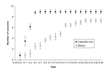
X. Xi, J. N. Griffin, S. Sun, Grasshoppers amensalistically suppress caterpillar performance and enhance plant biomass in an alpine meadow, Oikos, 122 (2013), 1049–1057. https://doi.org/10.1111/j.1600-0706.2012.00126.x doi: 10.1111/j.1600-0706.2012.00126.x
    [3] C. García, M. Rendueles, M. Díaz, Microbial amensalism in Lactobacillus casei and Pseudomonas taetrolens mixed culture, Bioprocess Biosyst. Eng., 40 (2017), 1111–1122. https://doi.org/10.1007/s00449-017-1773-3 doi: 10.1007/s00449-017-1773-3
    [4] J. P. Veiga, W. Wamiti, V. Polo, M. Muchai, Interphyletic relationships in the use of nesting cavities: Mutualism, competition and amensalism among hymenopterans and vertebrates, Naturwissenschaften, 100 (2013), 827–834. https://doi.org/10.1007/s00114-013-1082-x doi: 10.1007/s00114-013-1082-x
    [5] J. M. Gómez, A. González-Megías, Asymmetrical interactions between ungulates and phytophagous insects: Being different matters, Ecology, 83 (2002), 203–211. https://doi.org/10.1890/0012-9658(2002)083[0203:AIBUAP]2.0.CO;2 doi: 10.1890/0012-9658(2002)083[0203:AIBUAP]2.0.CO;2
    [6] Y. B. Hong, S. M. Chen, F. D. Chen, On the existence of positive periodic solution of an amensalism model with Beddington-DeAngelis functional response, WSEAS Trans. Math., 21 (2022), 572-579. https://doi.org/10.37394/23206.2022.21.64 doi: 10.37394/23206.2022.21.64
    [7] X. He, Z. Zhu, J. Chen, F. Chen, Dynamical analysis of a Lotka Volterra commensalism model with additive Allee effect, Open Math., 20 (2022), 646–665. https://doi.org/10.1515/math-2022-0055 doi: 10.1515/math-2022-0055
    [8] L. L. Xu, Y. L. Xue, Q. F. Lin, C. Q. Lei, Global attractivity of symbiotic model of commensalism in four populations with Michaelis-Menten type harvesting in the first commensal populations, Axioms, 11 (2022), 337. https://doi.org/10.3390/axioms11070337 doi: 10.3390/axioms11070337
    [9] G. C. Sun, Qualitative analysis on two populations amensalism model, J. Jiamusi Univ., 21 (2003), 283–286.
    [10] Z. F. Zhu, Y. A. Li, F. Xu, Mathematical analysis on commensalism Lotka-Volterra model of populations, J. Chongqing Inst. Technol., 8 (2008), 100–101.
    [11] Z. Wei, Y. Xia, T. Zhang, Stability and bifurcation analysis of an amensalism model with weak Allee effect, Qualitative Theory Dyn. Syst., 19 (2020). https://doi.org/10.1007/s12346-020-00341-0
    [12] D. Luo, Q. Wang, Global dynamics of a Holling-II amensalism system with nonlinear growth rate and Allee effect on the first species, Int. J. Bifurcation Chaos, 31 (2021), 2150050. https://doi.org/10.1142/S0218127421500504 doi: 10.1142/S0218127421500504
    [13] D. Luo, Q. Wang, Global dynamics of a Beddington-DeAngelis amensalism system with weak Allee effect on the first specie, Appl. Math. Comput., 408 (2021), 126368. https://doi.org/10.1016/j.amc.2021.126368 doi: 10.1016/j.amc.2021.126368
    [14] M. Zhao, Y. Du, Stability and bifurcation analysis of an amensalism system with Allee effect, Adv. Differ. Equations, 2020 (2020). https://doi.org/10.1186/s13662-020-02804-9
    [15] H. Liu, H. Yu, C. Dai, H. Deng, Dynamical analysis of an aquatic amensalism model with non-selective harvesting and Allee effect, Math. Biosci. Eng., 18 (2021), 8857–8882. https://doi.org/10.3934/mbe.2021437 doi: 10.3934/mbe.2021437
    [16] R. Wu, A two species amensalism model with non-monotonic functional response, Commun. Math. Biol. Neurosci., 2016 (2016), 19. https://doi.org/10.28919/cmbn/2839 doi: 10.28919/cmbn/2839
    [17] Y. B. Chong, S. M. Chen, F. D. Chen, On the existence of positive periodic solution of an amensalism model with Beddington-DeAngelis functional response, WSEAS Trans. Math., 21 (2022), 572–579. https://doi.org/10.37394/23206.2022.21.64 doi: 10.37394/23206.2022.21.64
    [18] X. Guan, F, Chen, Dynamical analysis of a two species amensalism model with Beddington-DeAngelis functional response and Allee effect on the second species, Nonlinear Anal. Real World Appl., 48 (2019), 71–93. https://doi.org/10.1016/j.nonrwa.2019.01.002 doi: 10.1016/j.nonrwa.2019.01.002
    [19] Y. Liu, L. Zhao, X. Huang, H. Deng, Stability and bifurcation analysis of two species amensalism model with Michaelis-Menten type harvesting and a cover for the first species, Adv. Differ. Equations, 2018 (2018). https://doi.org/10.1186/s13662-018-1752-2
    [20] M. Zhao, Y. Ma, Y. Du, Global dynamics of an amensalism system with Michaelis-Menten type harvesting, Electron. Res. Arch., 31 (2022), 549–574. https://doi.org/10.3934/era.2023027 doi: 10.3934/era.2023027
    [21] Q. Zhou, F. Chen, S. Lin, Complex dynamics analysis of a discrete amensalism system with a cover for the first species, Axioms, 11 (2022), 365. https://doi.org/10.3390/axioms11080365 doi: 10.3390/axioms11080365
    [22] C. Lei, Dynamic behaviors of a stage structure amensalism system with a cover for the first species, Adv. Differ. Equations, 2018 (2018). https://doi.org/10.1186/s13662-018-1729-1
    [23] Y. Liu, L. Zhao, X. Huang, H. Deng, Stability and bifurcation analysis of two species amensalism model with Michaelis-Menten type harvesting and a cover for the first species, Adv. Differ. Equations, 2018 (2018). https://doi.org/10.1186/s13662-018-1752-2
    [24] X. D. Xie, F. D. Chen, M. X. He, Dynamic behaviors of two species amensalism model with a cover for the first species, J. Math. Comput. Sci., 16 (2016), 395–401. http://dx.doi.org/10.22436/jmcs.016.03.09 doi: 10.22436/jmcs.016.03.09
    [25] L. Y. Zanette, A. F. White, M. C. Allen, M. Clinchy, Perceived predation risk reduces the number of offspring songbirds produce per year, Science, 334 (2011), 1398–1401. https://doi.org/10.1126/science.1210908 doi: 10.1126/science.1210908
    [26] K. H. Elliott, G. S. Betini, D. R. Norris, Experimental evidence for within- and cross-seasona effects of fear on survival and reproduction, J. Anim. Ecol., 85 (2010), 507–515. https://doi.org/10.1111/1365-2656.12487 doi: 10.1111/1365-2656.12487
    [27] X. Wang, L. Zanette, X. Zou, Modelling the fear effect in predator-prey interactions, J. Math. Biol., 73 (2016), 1179–1204. https://doi.org/10.1007/s00285-016-0989-1 doi: 10.1007/s00285-016-0989-1
    [28] A. A. Thirthar, S. J. Majeed, M. A. Alqudah, P. Panja, T. Abdeljawad, Fear effect in a predator-prey model with additional food, prey refuge and harvesting on super predator, Chaos Solitons Fractals, 159 (2022), 112091. https://doi.org/10.1016/j.chaos.2022.112091 doi: 10.1016/j.chaos.2022.112091
    [29] K. Sarkar, S. Khajanchi, Impact of fear effect on the growth of prey in a predator-prey interaction model, Ecol. Complexity, 42 (2020), 100826. https://doi.org/10.1016/j.ecocom.2020.100826 doi: 10.1016/j.ecocom.2020.100826
    [30] J. Chen, X. He, F. Chen, The influence of fear effect to a discrete-time predator-prey system with predator has other food resource, Mathematics, 9 (2021), 865. https://doi.org/10.3390/math9080865 doi: 10.3390/math9080865
    [31] D. L. Ogada, M. E. Gadd, R. S. Ostfeld, T. P. Young, F. Keesing, Impacts of large herbivorous mammals on bird diversity and abundance in an African savanna, Oecologia, 156 (2008), 387–397. https://doi.org/10.1007/s00442-008-0994-1 doi: 10.1007/s00442-008-0994-1
    [32] Q. Zhou, F. Chen, Dynamical analysis of a discrete amensalism system with the Beddington-DeAngelis functional response and Allee effect for the unaffected species, Qualitative Theory Dyn. Syst., 22 (2023), 16. https://doi.org/10.1007/s12346-022-00716-5 doi: 10.1007/s12346-022-00716-5
    [33] P. Panday, N. Pal, S. Samanta, J. Chattopadhyay, A three species food chain model with fear induced trophic cascade, Int. J. Appl. Comput. Math., 5 (2019), 1–26. https://doi.org/10.1007/s40819-019-0688-x doi: 10.1007/s40819-019-0688-x
    [34] S. K. Sasmal, Y. Takeuchi, Dynamics of a predator-prey system with fear and group defense, J. Math. Anal. Appl., 481 (2020), 123471. https://doi.org/10.1016/j.jmaa.2019.123471 doi: 10.1016/j.jmaa.2019.123471
    [35] H. Zhang, Y. Cai, S. Fu, W. Wang, Impact of the fear effect in a prey-predator model incorporating a prey refuge, Appl. Math. Comput., 356 (2019), 328–337. https://doi.org/10.1016/j.amc.2019.03.034 doi: 10.1016/j.amc.2019.03.034
    [36] H. Singh, J. Dhar, H. S. Bhatti, Discrete-time bifurcation behavior of a prey-predator system with generalized predator, Adv. Differ. Equations, 2015 (2015), 206. https://doi.org/10.1186/s13662-015-0546-z doi: 10.1186/s13662-015-0546-z
    [37] R. Banerjee, P. Das, D. Mukherjee, Stability and permanence of a discrete-time two-prey one-predator system with Holling type-III functional response, Chaos Solitons Fractals, 117 (2018), 240–248. https://doi.org/10.1016/j.chaos.2018.10.032 doi: 10.1016/j.chaos.2018.10.032
    [38] Q. Din, Complexity and chaos control in a discrete-time prey-predator mode, Commun. Nonlinear Sci. Numer. Simul., 49 (2018), 113–134. https://doi.org/10.1016/j.cnsns.2017.01.025 doi: 10.1016/j.cnsns.2017.01.025
    [39] H. Jiang, T.D. Rogers, The discrete dynamics of symmetric competition in the plane, J. Math. Biol., 25 (1978), 573–596. https://doi.org/10.1007/BF00275495 doi: 10.1007/BF00275495
    [40] F. Chen, Permanence for the discrete mutualism model with time delays, Math. Comput. Modell., 47 (2008), 431–435. https://doi.org/10.1016/j.mcm.2007.02.023 doi: 10.1016/j.mcm.2007.02.023
    [41] D. C. Liaw, Application of center manifold reduction to nonlinear system stabilization, Appl. Math. Comput., 91 (1998), 243-258. https://doi.org/10.1016/S0096-3003(97)10021-2 doi: 10.1016/S0096-3003(97)10021-2
    [42] S. Wiggins, Introduction to Applied Nonlinear Dynamical Systems and Chaos, Springer Science and Business Media, 2003.
    [43] C. Robinson, Dynamical Systems: Stability, Symbolic Dynamics and Chaos, CRC Press, 1998.
  • This article has been cited by:

    1. Jinhong Wang, Yanting Xu, Factors influencing the transition of China's economic growth momentum, 2024, 6, 2689-3010, 220, 10.3934/NAR.2024010
    2. Barış Armutcu, Ahmet Tan, Shirie Pui Shan Ho, Matthew Yau Choi Chow, Kimberly C. Gleason, The effect of bank artificial intelligence on consumer purchase intentions, 2024, 0368-492X, 10.1108/K-01-2024-0145
    3. Ayse Basak Cinar, Stephane Bilodeau, Incorporating AI into the Inner Circle of Emotional Intelligence for Sustainability, 2024, 16, 2071-1050, 6648, 10.3390/su16156648
    4. Murali Mohana Kumara Varma Mantena, Giri Murugan, 2025, 3281, 0094-243X, 020031, 10.1063/5.0247131
    5. Ahuod Hameed Alsubhi, Emad Sami Jaha, Front-to-Side Hard and Soft Biometrics for Augmented Zero-Shot Side Face Recognition, 2025, 25, 1424-8220, 1638, 10.3390/s25061638
    6. Hui Qi, Yue Liu, Hanzi Chen, Pierre Failler, The Impact of Enterprise Digitalization on Green Total Factor Productivity: Evidence from Chinese Provinces, 2025, 17, 2071-1050, 3707, 10.3390/su17083707
  • Reader Comments
  • © 2024 the Author(s), licensee AIMS Press. This is an open access article distributed under the terms of the Creative Commons Attribution License (http://creativecommons.org/licenses/by/4.0)
通讯作者: 陈斌, bchen63@163.com
  • 1. 

    沈阳化工大学材料科学与工程学院 沈阳 110142

  1. 本站搜索
  2. 百度学术搜索
  3. 万方数据库搜索
  4. CNKI搜索

Metrics

Article views(1683) PDF downloads(87) Cited by(1)

Article outline

Other Articles By Authors

/

DownLoad:  Full-Size Img  PowerPoint
Return
Return

Catalog