


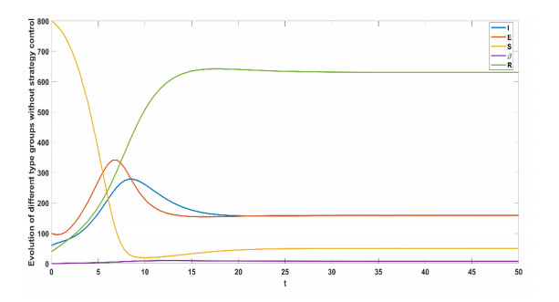
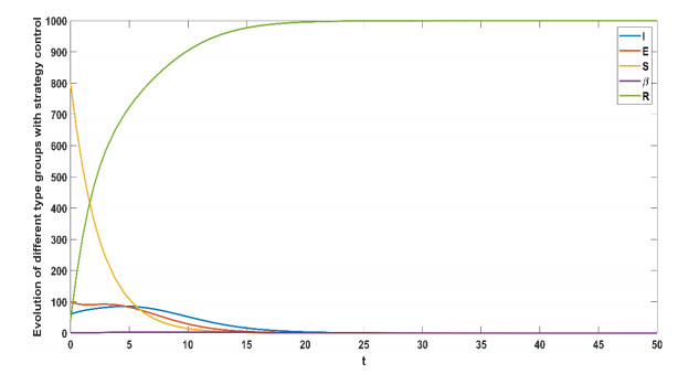
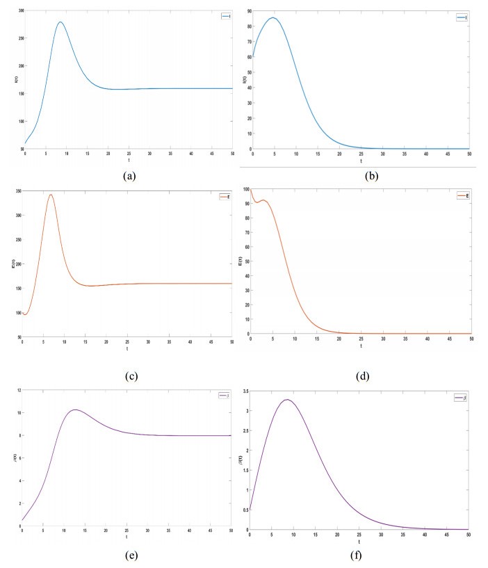
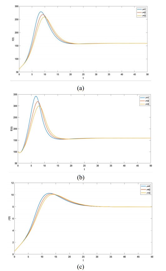
In emergencies similar to virus spreading in an epidemic model, panic can spread in groups, which brings serious bad effects to society. To explore the transmission mechanism and decision-making behavior of panic, a government strategy was proposed in this paper to control the spread of panic. First, based on the SEIR epidemiological model, considering the delay effect between susceptible and exposed individuals and taking the infection rate of panic as a time-varying variable, a SEIR delayed panic spread model was established and the basic regeneration number of the proposed model was calculated. Second, the control strategy was expressed as a state delayed feedback and solved using the exact linearization method of nonlinear control system; the control law for the system was determined, and its stability was proven. The aim was to eradicate panic from the group so that the recovered group tracks the whole group asymptotically. Finally, we simulated the proposed strategy of controlling the spread of panic to illustrate our theoretical results.
Citation: Rongjian Lv, Hua Li, Qiubai Sun, Bowen Li. Model of strategy control for delayed panic spread in emergencies[J]. Mathematical Biosciences and Engineering, 2024, 21(1): 75-95. doi: 10.3934/mbe.2024004
| [1] | Shuyue Ma, Jiawei Sun, Huimin Yu . Global existence and stability of temporal periodic solution to non-isentropic compressible Euler equations with a source term. Communications in Analysis and Mechanics, 2023, 15(2): 245-266. doi: 10.3934/cam.2023013 |
| [2] | Shu Wang . Global well-posedness and viscosity vanishing limit of a new initial-boundary value problem on two/three-dimensional incompressible Navier-Stokes equations and/or Boussinesq equations. Communications in Analysis and Mechanics, 2025, 17(2): 582-605. doi: 10.3934/cam.2025023 |
| [3] | Zhigang Wang . Serrin-type blowup Criterion for the degenerate compressible Navier-Stokes equations. Communications in Analysis and Mechanics, 2025, 17(1): 145-158. doi: 10.3934/cam.2025007 |
| [4] | Reinhard Racke . Blow-up for hyperbolized compressible Navier-Stokes equations. Communications in Analysis and Mechanics, 2025, 17(2): 550-581. doi: 10.3934/cam.2025022 |
| [5] | Hongxia Lin, Sabana, Qing Sun, Ruiqi You, Xiaochuan Guo . The stability and decay of 2D incompressible Boussinesq equation with partial vertical dissipation. Communications in Analysis and Mechanics, 2025, 17(1): 100-127. doi: 10.3934/cam.2025005 |
| [6] | Yang Liu, Xiao Long, Li Zhang . Long-time dynamics for a coupled system modeling the oscillations of suspension bridges. Communications in Analysis and Mechanics, 2025, 17(1): 15-40. doi: 10.3934/cam.2025002 |
| [7] | Fangyuan Dong . Multiple positive solutions for the logarithmic Schrödinger equation with a Coulomb potential. Communications in Analysis and Mechanics, 2024, 16(3): 487-508. doi: 10.3934/cam.2024023 |
| [8] | Zhen Wang, Luhan Sun . The Allen-Cahn equation with a time Caputo-Hadamard derivative: Mathematical and Numerical Analysis. Communications in Analysis and Mechanics, 2023, 15(4): 611-637. doi: 10.3934/cam.2023031 |
| [9] | Rui Sun, Weihua Deng . A generalized time fractional Schrödinger equation with signed potential. Communications in Analysis and Mechanics, 2024, 16(2): 262-277. doi: 10.3934/cam.2024012 |
| [10] | Chunyou Sun, Junyan Tan . Attractors for a Navier–Stokes–Allen–Cahn system with unmatched densities. Communications in Analysis and Mechanics, 2025, 17(1): 237-262. doi: 10.3934/cam.2025010 |
In emergencies similar to virus spreading in an epidemic model, panic can spread in groups, which brings serious bad effects to society. To explore the transmission mechanism and decision-making behavior of panic, a government strategy was proposed in this paper to control the spread of panic. First, based on the SEIR epidemiological model, considering the delay effect between susceptible and exposed individuals and taking the infection rate of panic as a time-varying variable, a SEIR delayed panic spread model was established and the basic regeneration number of the proposed model was calculated. Second, the control strategy was expressed as a state delayed feedback and solved using the exact linearization method of nonlinear control system; the control law for the system was determined, and its stability was proven. The aim was to eradicate panic from the group so that the recovered group tracks the whole group asymptotically. Finally, we simulated the proposed strategy of controlling the spread of panic to illustrate our theoretical results.
In this paper, we study the 2D steady compressible Prandtl equations in {x>0,y>0}:
| {u∂xu+v∂yu−1ρ∂2yu=−∂xP(ρ)ρ,∂x(ρu)+∂y(ρv)=0,u|x=0=u0(y),limy→∞u=U(x),u|y=0=v|y=0=0, | (1.1) |
where (u,v) is velocity field, ρ(x) and U(x) are the traces at the boundary {y=0} of the density and the tangential velocity of the outer Euler flow. The states ρ,U satisfy the Bernoulli law
| U∂xU+∂xP(ρ)ρ=0. | (1.2) |
The pressure P(ρ) is a strictly increasing function of ρ with 0<ρ0≤ρ≤ρ1 for some positive constants ρ0 and ρ1.
In this paper, we assume that the pressure satisfies the favorable pressure gradient ∂xP≤0, which implies that
| ∂xρ≤0. |
The boundary layer is a very important branch in fluid mechanics. Ludwig Prandtl [14] first proposed the related theory of the boundary layer in 1904. Since then, many scholars have devoted themselves to studying the mathematical theory of the boundary layer [1,7,8,9,11,12,17,18,19,21,22,23,24,26,27]. For more complex fluids, such as compressible fluids, one can refer to [19,20,28] and the references therein for more details. Here, for our purposes, we only list some relevant works.
There are three very natural problems about the steady boundary layer: (ⅰ) Boundary layer separation, (ⅱ) whether Oleinik's solutions are smooth up to the boundary for any x>0 and (ⅲ) vanishing viscosity limit of the steady Navier-Stokes system. Next, we will introduce the relevant research progress in these three aspects. The separation of the boundary layer is one of the very important research contents in the boundary layer theory. [17]. The earliest mathematical theory in this regard was proposed by Caffarelli and E in an unpublished paper [25]. Their results show that the existence time x∗ of the solutions to the steady Prandtl equations in the sense of Oleinik is finite under the adverse pressure gradient. Moreover, the family uμ(x,y)=μ−12u(x∗−μx,μ14y) is compact in C0(R2+). Later, Dalibard and Masmoudi [4] proved the solution behaves near the separation as ∂yu(x,0)∼(x∗−x)12 for x<x∗. Shen, Wang and Zhang [18] found that the solution near the separation point behaves like ∂yu(x,y)∼(x∗−x)14 for x<x∗. The above work further illustrates that the boundary layer separation is a very complex phenomenon. Recently, there were also some results about the steady compressible boundary layer separation [28]. The authors found that if the heat transfer in the boundary layer disappeared, then the singularity would be the same as that in the incompressible case. There is still relatively little mathematical theory on the separation of unsteady boundary layers. This is because back-flow and separation no longer occur simultaneously. When the boundary layer back-flow occurs, the characteristics of the boundary layer will continue to maintain for a period of time. Therefore, it is very important to study the back-flow point for further research on separation. Recently, Wang and Zhu [21] studied the back-flow problem of the two-dimensional unsteady boundary layer, which is a important work. It is very interesting to further establish the mathematical theory of the unsteady boundary layer separation.
Due to degenerate near the boundary, the high regularity of the solution of the boundary layer equation is a very difficult and meaningful work. In a local time 0<x<x∗≪1, Guo and Iyer [6] studied the high regularity of of the Prandtl equations. Oleinik and Samokhin [13] studied the existence of solutions of steady Prandtl equations and Wang and Zhang [23] proved that Oleinik's solutions are smooth up to the boundary y=0 for any x>0. The goal of this paper is to prove the global C∞ regularity of the two-dimensional steady compressible Prandtl equations. Recently, Wang and Zhang [24] found the explicit decay for general initial data with exponential decay by using the maximum principle.
In addition, in order to better understand the relevant background knowledge, we will introduce some other related work. As the viscosity goes to zero, the solutions of the three-dimensional evolutionary Navier-Stokes equations to the solutions of the Euler equations are an interesting problem. Beirão da Veiga and Crispo [2] proved that in the presence of flat boundaries convergence holds uniformly in time with respect to the initial data's norm. For the non-stationary Navier-Stokes equations in the 2D power cusp domain, the formal asymptotic expansion of the solution near the singular point is constructed and the constructed asymptotic decomposition is justified in [15,16] by Pileckas and Raciene.
Before introducing the main theorem, we introduce some preliminary knowledge. To use the von Mises transformation, we set
| ˜u(x,y)=ρ(x)u(x,y),˜v(x,y)=ρ(x)v(x,y),˜u0(y)=ρ(0)u0(y), |
then we find that (˜u,˜v) satisfies:
| {˜u∂x˜u+˜v∂y˜u−∂2y˜u−∂xρρ˜u2=−ρ∂xP(ρ),∂x˜u+∂y˜v=0,˜u|x=0=˜u0(y),limy→∞˜u=ρ(x)U(x),˜u|y=0=˜v|y=0=0. | (1.3) |
By the von Mises transformation
| x=x,ψ(x,y)=∫y0˜u(x,z)dz,w=˜u2, | (1.4) |
| ∂x˜u=∂xω2√ω+∂ψω∂xψ2√ω,∂y˜u=∂ψω2,∂2y˜u=√ω∂2ψω2, | (1.5) |
and (1.3)–(1.5), we know that w(x,ψ) satisfies:
| ∂xw−√w∂2ψw−2∂xρρw=−2ρ∂xP(ρ), | (1.6) |
with
| w(x,0)=0,w(0,ψ)=w0(ψ),limψ→+∞w=(ρ(x)U(x))2. | (1.7) |
In addition, we have
| 2∂y˜u=∂ψw,2∂2y˜u=√w∂2ψw. | (1.8) |
In [5], Gong, Guo and Wang studied the existence of the solutions of system (1.1) by using the von Mises transformation and the maximal principle proposed by Oleinik and Samokhin in [13]. Specifically, they proved that:
Theorem 1.1. If the initial data u0 satisfies the following conditions:
| u∈C2,αb([0,+∞))(α>0),u(0)=0,∂yu(0)>0,∂yu(y)≥0fory∈[0,+∞),limy→+∞u(y)=U(0)>0,ρ−1(0)∂2yu(y)−ρ−1(0)∂xP(0)=O(y2) | (1.9) |
and ρ∈C2([0,X0]), then there exists 0<X≤X0 such that system (1.1) admits a solution u∈C1([0,X)×R+). The solution has the following properties:
(i) u is continuous and bounded in [0,X]×R+; ∂yu,∂2yu are continuous and bounded in [0,X)×R+; v,∂yv,∂xu are locally bounded in [0,X)×R+.
(ii) u(x,y)>0 in [0,X)×R+ and for any ˉx<X, there exists y0,m>0 such that for all (x,y)∈[0,ˉx]×[0,y0],
| ∂yu(x,y)≥m>0. |
(iii) if ∂xP≤0(∂xρ≤0), then
| X=+∞. |
Remarks 1.2. u∈C2,αb([0,+∞))(α>0) means that u is Hölder continuity and bounded.
This theorem shows that under the favorable pressure gradient, the solution is global-in-x. However, if the pressure is an adverse pressure gradient, then boundary layer separation will occur. Xin and Zhang [26] studied the global existence of weak solutions of unsteady Prandtl equations under the favorable pressure gradient. For the unsteady compressible Prandtl equation, similar results are obtained in [3]. Recently, Xin, Zhang and Zhao [27] proposed a direct proof of the existence of global weak solutions of the Prandtl equation. The key content of this paper is that they have studied the uniqueness and regularity of weak solutions. This method can be applied to the compressible Prandtl equation.
Our main results are as follows:
Theorem 1.3. If u is a solution for equation (1.1) in Theorem 1.1, assume u0 satisfies the condition (1.9) and the known function ρ and ∂xP are smooth. Then, there exists a constant C>0 depending only on ε,X,u0,P(ρ),k,m such that for any (x,y)∈[ε,X]×[0,+∞),
| |∂kx∂myu(x,y)|≤C, |
where X,ε are positive constants with ε<X and m,k are any positive integers.
Remarks 1.4. Our methods may be used to other related models. There are similar results for the magnetohydrodynamics boundary layer and the thermal boundary layer. This work will be more difficult due to the influence of temperature and the magnetic field.
Due to the degeneracy near the boundary ψ=0, the proof of the main result is divided into two parts, Theorem 1.5 and Theorem 1.6. This is similar to the result of the incompressible boundary layer, despite the fluid being compressible and the degeneracy near the boundary. Different from the incompressible case [23], we have no divergence-free conditions, which will bring new terms. It is one of the difficulties in this paper to deal with these terms. Now, we will briefly introduce our proof framework. First, we prove the following theorem in the domain [ε,X]×[0,Y1] for a small Y1. The key ingredients of proof is that we employ interior priori estimates and the maximum principle developed by Krylov [10].
Theorem 1.5. If u is a solution for equation (1.1) in Theorem 1.1, assume u0 satisfies the condition (1.9) and the known function ρ and ∂xP are smooth. Then, there exists a small constant Y1>0 and a large constant C>0 depending only on ε,X,Y1,u0,P(ρ),k,m such that for any (x,y)∈[ε,X]×[0,Y1],
| |∂kx∂myu(x,y)|≤C, |
where X,ε are positive constants with ε<X and m,k are any positive integers.
Next, we prove the following theorem in the domain [ε,X]×[Y2,+∞) for a small positive constant Y2. The key of proof is that we prove (1.6) is a uniform parabolic equation in the domain [ε,X]×[Y2,+∞) in Section 4. Once we have (1.6) is a uniform parabolic equation, the global C∞ regularity of the solution is a direct result of interior Schauder estimates and classical parabolic regularity theory. The proof can be given similarly to the steady incompressible boundary layer. For the sake of simplicity of the paper, more details can be found in [23] and we omit it here.
Theorem 1.6. If u is a solution for equation (1.1) in Theorem 1.1, assume u0 satisfies the condition (1.9) and the known function ρ and ∂xP are smooth. Then, there exists a constant Y0>0 such that for any constant Y2∈(0,Y0), there exists a constant C>0 depending only on ε,X,Y2,u0,P(ρ),k,m such that for any (x,y)∈[ε,X]×[Y2,+∞),
| |∂kx∂myu(x,y)|≤C, |
where X,ε are positive constants with ε<X and m,k are any positive integers.
Therefore, Theorem 1.3 can be directly proven by combining Theorem 1.5 with Theorem 1.6.
The organization of this paper is as follows. In Section 2, we study lower order and higher order regularity estimates. In Section 3, we prove Theorem 1.5 in the domain near y=0 by transforming back to the original coordinates (x,y). In Section 4, we prove (1.6) is a uniform parabolic equation by using the maximum principle and we also prove the Theorem 1.3.
In this subsection, we study the lower order regularity estimates using the standard interior a priori estimates developed by Krylov [10].
Lemma 2.1. If u is a solution for equation (1.1) in Theorem 1.1, assume u0 satisfies the condition (1.9)and the known function ρ and ∂xP are smooth. Assume 0<ε<X, then there exists some positive constants δ1>0 and C independent of ψ such that for any (x,ψ)∈[ε,X]×[0,δ1],
| |∂xw(x,ψ)|≤Cψ. |
Proof. Due to Lemma 2.1 in [5] (or Theorem 2.1.14 in [13]), there exists δ1>0 for any (x,ψ)∈[0,X]×[0,δ1], such that for some α∈(0,12) and positive constants m,M (we assume δ1<1),
| |∂xw|≤Cψ12+α,0<m<∂ψw<M,mψ<w<Mψ. | (2.1) |
By (1.6), we obtain
| ∂x∂xw−√w∂2ψ∂xw=(∂xw)22w+2ρ∂xP∂xw2w+∂xρρ∂xw+2∂x(∂xρρ)w−2∂x[ρ∂xP]. |
Take a smooth cutoff function 0≤ϕ(x)≤1 in [0,X] such that
| ϕ(x)=1,x∈[ε,X],ϕ(x)=0,x∈[0,ε2], |
then
| ∂x[∂xwϕ(x)]−√w∂2ψ[∂xwϕ(x)]=(∂xw)22wϕ(x)+2ρ∂xP∂xw2wϕ(x)+∂xρρ∂xwϕ(x)+2∂x(∂xρρ)wϕ(x)−2∂x(ρ∂xP)ϕ(x)+∂xw∂xϕ(x):=W. |
Combining with (2.1), we know
| |W|≤Cψ2α+Cψα−12+Cψα+12+Cψ+C≤Cψα−12. | (2.2) |
We take φ(ψ)=μ1ψ−μ2ψ1+β with constants μ1,μ2, then by (2.1) and (2.2), we get
| ∂x[∂xwϕ(x)−φ]−√w∂2ψ[∂xwϕ(x)−φ]≤|W|−μ2√wβ(1+β)ψβ−1≤Cψα−12−μ2√mβ(1+β)ψβ−12. |
By taking μ2 sufficiently large and α=β, for (x,ψ)∈(0,X]×(0,δ1), we have
| ∂x[∂xwϕ(x)−φ]−√w∂2ψ[∂xwϕ(x)−φ]<0. |
For any ψ∈[0,δ1], let μ1≥μ2, and we have
| (∂xwϕ−φ)(0,ψ)≤0, |
and take μ1 large enough depending on M,δ1,μ2 such that
| (∂xwϕ−φ)(x,δ1)≤Mδ12+α1−μ1δ1+μ2δ1+β1≤0. |
Since w(x,0)=0, we know that for any x∈[0,X],
| (∂xwϕ−φ)(x,0)=0. |
By the maximum principle, it holds in [0,X]×[0,δ1] that
| (∂xwϕ−φ)(x,ψ)≤0. |
Let δ1 be chosen suitably small, for (x,ψ)∈[ε,X]×[0,δ1], and we obtain
| ∂xw(x,ψ)≤μ1ψ−μ2ψ1+β≤μ12ψ. |
Considering −∂xwϕ−φ, the result −∂xw≤μ12ψ in [ε,X]×[0,δ1] can be proved similarly. This completes the proof of the lemma.
Lemma 2.2. If u is a solution for equation (1.1) in Theorem 1.1, assume u0 satisfies the condition (1.9) and the known function ρ and ∂xP are smooth. Assume 0<ε<X, then there exists some positive constants δ2>0 and C independent of ψ such that for any (x,ψ)∈[ε,X]×[0,δ2],
| |∂ψ∂xw(x,ψ)|≤C,|∂2xw(x,ψ)|≤Cψ−12,|∂2ψ∂xw(x,ψ)|≤Cψ−1. |
Proof. From Lemma 2.1, there exists δ1>0 such that for any (x,ψ)∈[ε2,X]×[0,δ1],
| |∂xw(x,ψ)|≤Cψ. |
Let Ψ0=min{23δ1,ε2}, for any (x0,ψ0)∈[ε,X]×(0,Ψ0], and we denote
| Ω={(x,ψ)|x0−ψ320≤x≤x0,12ψ0≤ψ≤32ψ0}. |
By the definition of Ψ0, we know Ω⊆[ε2,X]×[0,δ1], then it holds in Ω that
| |∂xw|≤Cψ. | (2.3) |
The following transformation f is defined:
| Ω→˜Ω:=[−1,0]˜x×[−12,12]˜ψ,(x,ψ)↦(˜x,˜ψ), |
where x−x0=ψ320˜x,ψ−ψ0=ψ0˜ψ.
Since ∂˜x=ψ320∂x,∂˜ψ=ψ0∂ψ, it holds in Ω that
| ∂˜x(ψ−10w)−ψ−120√w∂2˜ψ(ψ−10w)−2∂˜xρρ(ψ−10w)=−2ρ∂˜xPψ−10. |
Combining with (2.1), we get 0<c≤ψ−120√w≤C,|ψ−10w|≤C, and for any ˜z1,˜z2∈˜Ω,
| |ψ−120√w(˜z1)−ψ−120√w(˜z2)|=ψ−120|w(˜z1)−w(˜z2)|√w(˜z1)+√w(˜z2)≤Cψ0|˜z1−˜z2|ψ0=C|˜z1−˜z2|. |
This means that for any α∈(0,1), we have
| |ψ−120√w|Cα(˜Ω)≤C. |
Since P and ρ are smooth, we have
| |ρ−1∂˜xρ|C0,1([−1,0]˜x)+|ρ∂˜xPψ−10|C0,1([−1,0]˜x)≤C. |
By standard interior priori estimates (see Theorem 8.11.1 in [10] or Proposition 2.3 in [23]), we have
| |wψ−10|Cα([−12,0]˜x×[−14,14]˜ψ)+|∂2˜ψwψ−10|Cα([−12,0]˜x×[−14,14]˜ψ)≤C. | (2.4) |
Let f:=∂xwψ−10, which satisfies
| ∂˜xf−√wψ120∂2˜ψf−∂2˜ψw2√wψ120f−2∂˜xρρf=−2∂x[ρ∂˜xP]ψ−10+2∂x(∂˜xρρ)(ψ−10w). |
By (2.3), we have |f|≤C in ˜Ω. Due to
| |ψ120w−12(˜z1)−ψ120w−12(˜z2)|=ψ120|w(˜z1)−w(˜z2)w(˜z1)w(˜z2)|w−12(˜z1)+w−12(˜z2)≤C|˜z1−˜z2|, |
we have
| |ψ120w−12|Cα(˜Ω)≤C. | (2.5) |
Since
| ∂2˜ψw2√wψ120=∂2˜ψwψ−10ψ1202√w, |
which along with (2.4) and (2.5) gives
| |∂2˜ψw2√wψ120|Cα([−12,0]˜x×[−14,14]˜ψ)≤C. |
As before, by (2.4) and the density ρ and P are smooth, via the standard interior a priori estimates, it yield that
| |∂˜xf|L∞([−14,0]˜x×[−18,18]˜ψ)+|∂˜ψf|L∞([−14,0]˜x×[−18,18]˜ψ)+|∂2˜ψf|L∞([−14,0]˜x×[−18,18]˜ψ)≤C. |
Therefore, we obtain
| |∂2xw(x0,ψ0)|≤Cψ−120,|∂ψ∂xw(x0,ψ0)|≤C,|∂2ψ∂xw(x0,ψ0)|≤Cψ−10. |
This completes the proof of the lemma.
In this subsection, we study the higher order regularity estimates using the maximum principle. The two main results of this subsection are Lemma 2.3 and Lemma 2.7.
Lemma 2.3. If u is a solution for equation (1.1) in Theorem 1.1, assume u0 satisfies the condition (1.9) and the known function ρ and ∂xP are smooth. Assume 0<ε<X and k≥2, then there exists some positive constants δ>0 and C independent of ψ such that for any (x,ψ)∈[ε,X]×[0,δ],
| |∂kxw|≤Cψ,|∂ψ∂kxw|≤C,|∂2ψ∂kxw|≤Cψ−1. |
Proof. By Lemma 2.1 and Lemma 2.2, we may inductively assume that for 0≤j≤k−1, there holds that in [ε2,X]×[0,δ3] (assume δ3≪1),
| |∂ψ∂jxw|≤C,|∂2ψ∂jxw|≤Cψ−1,|∂jxw|≤Cψ,|∂jx√w|≤Cψ12,|∂kxw|≤Cψ−12. | (2.6) |
We will prove that there exists δ4<δ3 so that in [ε,X]×[0,δ4],
| |∂ψ∂kxw|≤C,|∂2ψ∂kxw|≤Cψ−1,|∂kxw|≤Cψ,|∂kx√w|≤Cψ12,|∂k+1xw|≤Cψ−12. | (2.7) |
The above results are deduced from the following Lemma 2.4, Lemma 2.5 and Lemma 2.6.
Lemma 2.4. If u is a solution for equation (1.1) in Theorem 1.1, assume u0 satisfies the condition (1.9) and the known function ρ and ∂xP are smooth. Assume that (2.6) holds, then there is a positive constant M1 for any (x,ψ)∈[7ε8,X]×[0,δ3] and 0<β≪1,
| |∂kxw|<M1ψ1−β,|∂kx√w|≤M1ψ12−β. |
Proof. Take a smooth cutoff function 0≤ϕ(x)≤1 in [0,X] such that
| ϕ(x)=1,x∈[7ε8,X],ϕ(x)=0,x∈[0,5ε8]. |
As in [23], fix any h<ε8. Set
| Ω={(x,ψ)|0<x≤X,0<ψ<δ3}, |
and let
(ⅰ) f=∂k−1xw(x−h,ψ)−∂k−1xw(x,ψ)−hϕ+Mψlnψ, (x,ψ)∈[5ε8,X]×[0,+∞),
(ⅱ) f=Mψlnψ, (x,ψ)∈[0,5ε8)×[ψ,+∞),
so we get f(x,0)=0, f(0,ψ)≤0. We know
| f(x,δ3)≤C(δ3)−12+Mδ3lnδ3≤0, |
where M is large enough. Then, by choosing the appropriate M, we know that the positive maximum of f cannot be achieved in the interior. Finally, the lemma can be proven by the arbitrariness of h.
Assume that there exists a point
| p0=(x0,ψ0)∈Ω, |
such that
| f(p0)=maxˉΩf>0. |
It is easy to know that
| x0>5ε8,∂k−1xw(x0−h,ψ0)<∂k−1xw(x0,ψ0). |
By (2.1), denote ξ=√m, we have
| −√w∂2ψ(Mψlnψ)=−M√wψ−1≤−ξMψ−12. | (2.8) |
By (1.6), a direct calculation gives
| ∂x∂k−1xw−√w∂2ψ∂k−1xw=−2∂k−1x(ρ∂xP)+k−2∑m=1Cmk−1(∂k−1−mx√w)∂2ψ∂mxw+(∂k−1x√w)∂2ψw+2k−1∑m=0Cmk−1∂k−1−mx(∂xρρ)∂mxw=−2∂k−1x(ρ∂xP)+k−2∑m=1Cmk−1(∂k−1−mx√w)∂2ψ∂mxw+∂k−1xw2√w∂xw√w+(∂k−1xw2√w)2ρ∂xP√w−(∂k−1xw2√w)2∂xρρw√w+2k−1∑m=0Cmk−1∂k−1−mx(∂xρρ)∂mxw+k−2∑m=0Cmk−2∂2ψw∂m+1xw∂k−2−mx12√w:=4∑i=1Ii |
and
| I1=−2∂k−1x(ρ∂xP)+k−2∑m=1Cmk−1(∂k−1−mx√w)∂2ψ∂mxw+∂k−1xw2√w∂xw√w,I2=ρ∂xPw∂k−1xw,I3=−∂xρρ∂k−1xw+2k−1∑m=0Cmk−1∂k−1−mx(∂xρρ)∂mxw,I4=k−2∑m=0Cmk−2∂2ψw∂m+1xw∂k−2−mx12√w. |
For x≥5ε8, we consider the following equality
| ∂xf1−√w(p1)∂2ψf1=√w(p1)−√w(p)−h∂2ψ∂k−1xw(p)+4∑i=11−h(Ii(p1)−Ii(p)), | (2.9) |
where
| f1=1−h(∂k−1xw(p1)−∂k−1xw(p)), |
with p1=(x−h,ψ),p=(x,ψ).
For any x≥5ε8, by (2.6), it is easy to conclude that
| |1−h(√w(p1)−√w(p))∂2ψ∂k−1xw(p)|≤Cψ−12,|1−h(I1(p1)−I1(p))|≤Cψ−12,|4∑i=31−h(Ii(p1)−Ii(p))|≤Cψ−12, | (2.10) |
where C is dependent on the parameter h.
Since
| 1−h(I2(p1)−I2(p))=f1⋅[ρ∂xPw(p1)]+∂k−1xw(p)1−h[ρ∂xPw(p1)−ρ∂xPw(p)], |
combining with (2.6), f1(p0)>0 and ∂xP≤0, it holds at p=p0 that
| 1−h(I2(p1)−I2(p0))≤C. | (2.11) |
Summing up (2.10) and (2.11), we conclude that at p=p0,
| ∂xf1−√w∂2ψf1≤C0ψ−12. |
This along with (2.8) shows that for x≥5ε8, it holds at p=p0 that
| ∂xf−√w∂2ψf≤Cψ−12−ξMψ−12. | (2.12) |
By taking M large enough, we have ∂xf(p0)−√w∂2ψf(p0)<0. By the definition of p0, we obtain
| ∂xf(p0)−√w∂2ψf(p0)≥0, |
which leads to a contradiction. Therefore, for M chosen as above and independent of h, we have
| maxˉΩf≤0. |
We can similarly prove that minˉΩf≥0 by replacing Mψlnψ in f with −Mψlnψ. By the arbitrariness of h, for any (x,ψ)∈(7ε8,X]×(0,δ3] we have
| |∂kxw|≤−Mψlnψ. |
Due to
| 2√w∂kx√w+k−1∑m=1Cmk(∂mx√w∂k−mx√w)=∂kx(√w√w)=∂kxw, | (2.13) |
which along with (2.6) shows that in (78ε,X]×(0,δ3],
| |√w∂kx√w|≤−Cψlnψ. |
Lemma 2.5. If u is a solution for equation (1.1) in Theorem 1.1, assume u0 satisfies the condition (1.9) and the known function ρ and ∂xP are smooth. Assume that (2.6) holds, then for any (x,ψ)∈[1516ε,X]×[0,δ3],
| |∂kxw|≤Cψ,|∂kx√w|≤Cψ12. |
Proof. Take a smooth cutoff function ϕ(x) so that
| ϕ(x)=1,x∈[15ε16,X],ϕ(x)=0,x∈[0,7ε8]. |
Set
| f=∂kxwϕ−μ1ψ+μ2ψ32−β |
with constants μ1,μ2. Let β be small enough in Lemma 2.4. Then it holds in [7ε8,X]×[0,δ3] that
| |∂kxw|≤Cψ1−β,|∂kx√w|≤Cψ12−β. | (2.14) |
We denote
| Ω={(x,ψ)|0<x≤X,0<ψ<δ3}. |
As in [23], we have f(x,0)=0, f(0,ψ)≤0 and f(x,δ3)≤0 by taking μ1 large depending on μ2. We claim that the maximum of f cannot be achieved in the interior.
By (1.6), we have
| ∂x∂kxw−√w∂2ψ∂kxw=−2∂kx(ρ∂xP)+k−1∑m=0Cmk(∂k−mx√w)∂2ψ∂mxw+2k∑m=0Cmk∂k−mx(∂xρρ)∂mxw, |
and
| ∂2ψ∂mxw=∂mx∂2ψw=∂mx(∂xw√w+2ρ∂xP√w−2∂xρρ√w). |
For any x≥7ε8, 0≤j≤k−1 and 0≤m≤k−1, from (2.6) and (2.14), we get
| |∂jxw|≤Cψ,|∂kxw|≤Cψ1−β,|∂k−mx√w|≤Cψ12−β. |
Then let β≪12, for 0≤m≤k−1 and x≥7ε8, we obtain
| |∂2ψ∂mxw|≤Cψ12−β+Cψ−12+Cψ12−β≤Cψ−12. |
Therefore, we conclude that for x≥7ε8,
| ∂x∂kxw−√w∂2ψ∂kxw≤C+Cψ−β+Cψ1−β≤Cψ−β. |
By the above inequality and (2.1), it holds at p=p0 that
| ∂xf−√w∂2ψf=∂x∂kxw−√w∂2ψ∂kxw+∂kxw∂xϕ−√w∂2ψ(−μ1ψ+μ2ψ32−β)≤C2ψ−β−ξμ2ψ−β, |
where ξ=(32−β)(12−β)√m>0. Then we have ∂xf−√w∂2ψf<0 in Ω by taking μ2 large depending on C2. This means that the maximum of f cannot be achieved in the interior. Therefore, we have
| maxˉΩf≤0. |
In the same way, we can prove that
| maxˉΩ−∂kxwϕ−μ1ψ+μ2ψ32−β≤0. |
So, for any (x,ψ)∈[1516ε,X]×[0,δ3], we have
| |∂kxw|≤μ1ψ−μ2ψ32−β≤μ1ψ. |
Combining with (2.6) and (2.13), it holds in [1516ε,X]×[0,δ3] that
| |∂kx√w|≤Cψ12. |
This completes the proof of the lemma.
Lemma 2.6. If u is a solution for equation (1.1) in Theorem 1.1, assume u0 satisfies the condition (1.9) and the known function ρ and ∂xP are smooth. Assume that (2.6) holds, then for any (x,ψ)∈[ε,X]×[0,δ4],
| |∂ψ∂kxw|≤C,|∂2ψ∂kxw|≤Cψ−1,|∂k+1xw|≤Cψ−12. |
Proof. By Lemma 2.5 and (2.6), for any (x,ψ)∈[1516ε,X]×[0,δ3],
| |∂jxw|≤Cψ,|∂jx√w|≤Cψ12,0≤j≤k. | (2.15) |
Set Ψ0=min{23δ3,ε16}, for (x0,ψ0)∈[ε,X]×(0,Ψ0], we denote
| Ω={(x,ψ)|x0−ψ320≤x≤x0,12ψ0≤ψ≤32ψ0}. |
A direct calculation gives
| ∂x∂kxw−√w∂2ψ∂kxw=−2∂kx(ρ∂xP)+∂kx√w∂2ψw+k−2∑m=1Cmk(∂k−mx√w)∂2ψ∂mxw+Ck−1k∂xw2√w∂2ψ∂k−1xw+2k∑m=0Cmk∂k−mx(∂xρρ)∂mxw. |
By (1.6), we obtain
| ∂2ψ∂mxw=∂mx∂2ψw=∂mx(∂xw√w+2ρ∂xP√w−2∂xρρ√w)=∂m+1xw√w+m∑l=1Clm∂m−l+1xw∂lx1√w+∂mx(2ρ∂xP√w)−∂mx(2∂xρρ√w), |
and
| ∂kx√w=∂k−1x∂xw2√w=∂kxw2√w+k−1∑l=1Clk−1∂k−1−l+1xw∂lx12√w, |
then
| ∂x∂kxw−√w∂2ψ∂kxw=−2∂kx(ρ∂xP)+k−2∑m=1Cmk(∂k−mx√w)∂2ψ∂mxw+∂kxw2√w∂2ψw+k−1∑l=1Clk−1∂k−1−l+1xw∂lx(12√w)∂2ψw+Ck−1k∂xw∂kxw2w+2k∑m=0Cmk∂k−mx(∂xρρ)∂mxw+Ck−1k∂xw2√w[k−1∑l=1Clk−1∂k−lxw∂lx1√w+∂k−1x(2ρ∂xP√w)−∂k−1x(2∂xρρ√w)]. |
The following transformation f is defined:
| Ω→˜Ω:=[−1,0]˜x×[−12,12]˜ψ,(x,ψ)↦(˜x,˜ψ), |
where x−x0=ψ320˜x,ψ−ψ0=ψ0˜ψ.
Let f=∂kxwψ−10, we get
| ∂˜xf−√wψ120∂2˜ψf−12√w∂2ψwψ320f−∂xw2wψ320f=−2ψ120∂kx(ρ∂xP)+ψ120k−2∑m=1Cmk(∂k−mx√w)∂2ψ∂mxw+ψ120k−1∑l=1Clk−1∂k−lxw(∂lx12√w)∂2ψw+2ψ120k∑m=0Cmk∂k−mx(∂xρρ)∂mxw+ψ120∂xw2√w[k−1∑l=1Clk−1∂k−lxw∂lx1√w+∂k−1x(2ρ∂xP√w)−∂k−1x(2∂xρρ√w)]:=F. |
From the proof of Lemma 2.2 and Lemma 2.6, we know that in ˜Ω for α∈(0,1),
| |f|≤C,0<c≤ψ−120√w≤C,|ψ−120√w|Cα(˜Ω)≤C. |
By (2.6), (2.15) and the equality
| ∂ψ(∂2ψ∂mxw)=∂ψ∂m+1xw√w−∂ψw∂m+1xw2(√w)3+m∑l=1Clm∂m−l+1x∂ψw∂lx1√w+m∑l=1Clm∂m−l+1xw∂lx∂ψw−2(√w)3+∂mx(ρ∂xP∂ψw−(√w)3)−∂mx(∂xρρ∂ψw√w), |
we can conclude that for j≤k−1 and m≤k−2,
| |∇˜x,˜ψ∂jx√w|≤Cψ120,|∇˜x,˜ψ∂jx(1√w)|≤Cψ−120,|∇˜x,˜ψ∂2ψ∂mxw|≤Cψ−120. |
Combining (2.4) with (2.5), we can obtain
| |12√w∂2ψwψ320+∂xw2wψ320|Cα(˜Ω)+|F|Cα(˜Ω)≤C. |
By the standard interior priori estimates, we obtain
| |∂˜xf|L∞([−14,0]˜x×[−18,18]˜ψ)+|∂˜ψf|L∞([−14,0]˜x×[−18,18]˜ψ)+|∂2˜ψf|L∞([−14,0]˜x×[−18,18]˜ψ)≤C. |
Therefore, this means that
| |∂k+1xw(x0,ψ0)|≤Cψ−120,|∂ψ∂kxw(x0,ψ0)|≤C,|∂2ψ∂kxw(x0,ψ0)|≤Cψ−10. |
Since (x0,ψ0) is arbitrary, this completes the proof of the lemma.
Lemma 2.7. If u is a solution for equation (1.1) in Theorem 1.1, assume u0 satisfies the condition (1.9) and the known function ρ and ∂xP are smooth. Assume 0<ε<X and integer m,k≥0, then there exists a positive constant δ>0 such that for any (x,ψ)∈[ε,X]×[0,δ],
| |∂mψ∂kxw|≤Cψ1−m. | (2.16) |
Proof. From Lemma 2.1, (2.1), Lemma 2.2 and Lemma 2.3, a direct calculation can prove that
| |∂kx1√w|≤Cψ−12,|∂kx∂ψ1√w|≤Cψ−32,|∂kx∂2ψ1√w|≤Cψ−52, |
and (2.16) holds for m=0,1,2. Then for 0≤m≤j with j≥1, we inductively assume that
| |∂mψ∂kxw|≤Cψ1−m,|∂kx∂mψ1√w|≤Cψ−12−m. | (2.17) |
In the next part, we will prove that (2.17) still holds for m=j+1.
By (1.6), we obtain
| ∂j+1ψ∂kxw=∂j−1ψ∂kx∂2ψw=∂kx∂j−1ψ(∂xw√w+2ρ∂xP√w−2∂xρρw√w)=∂kx(j−1∑i=0Cij−1∂j−1−iψ∂xw∂iψ1√w+2ρ∂xP∂j−1ψ1√w−2∂xρρj−1∑i=0Cij−1∂j−1−iψw∂iψ1√w). |
Combining with (2.17), we get
| |∂j+1ψ∂kxw|≤Cψ32−j+Cψ12−j+Cψ32−j≤Cψ12−j. | (2.18) |
By straight calculations, we get
| 0=∂kx∂j+1ψ(1√w1√ww)=∂kx[2√w∂j+1ψ1√w+j∑i=1j+1−i∑l=0Cij+1Clj+1−i(∂iψ1√w)(∂lψ1√w)∂j+1−l−iψw+j∑l=0Clj+11√w(∂lψ1√w)∂j+1−lψw]. |
Combining the above equality with (2.17), we can conclude that
| |∂kx∂j+1ψ1√w|≤Cψ−32−j. |
This completes the proof of the lemma.
In this section, we will prove the regularity of the solution u in the domain
| {(x,ψ)|ε≤x≤X,0≤y≤Y1}. |
Proof of Theorem 1.5:
Proof. For the convenience of proof, we denote
| (˜x,ψ)=(x,∫y0˜udy). |
A direct calculation gives (see P13 in [23])
| ∂y=√w∂ψ,∂x=∂˜x+∂xψ(x,y)∂ψ,∂xψ=12√w∫ψ0w−32∂˜xwdψ. |
By (2.1) and Lemma 2.3, we have |∂xψ|≤Cψ. Due to ∂y=√w∂ψ, we obtain
| ∂kx2∂y˜u=(∂˜x+∂xψ∂ψ)k∂ψw,∂kx2∂2y˜u=(∂˜x+∂xψ∂ψ)k(∂˜xw+2ρ∂xP−2∂xρρw)=(∂˜x+∂xψ∂ψ)k(∂˜xw)+2∂k˜x(ρ∂xP)−2(∂xρρ)(∂˜x+∂xψ∂ψ)kw−2∂k˜x(∂xρρ)w. |
By |∂xψ|≤Cψ and Lemma 2.7, we obtain that Theorem 1.5 holds for m=0,1,2,
| |∂kx∂y˜u|+|∂kx∂2y˜u|≤C. | (3.1) |
We inductively assume that for any integer k and m≥1,
| |∂kx∂jy˜u|≤C,j≤m. | (3.2) |
A direct calculation gives
| ∂kx∂m+1y˜u=∂kx∂m−1y∂2y˜u=∂kx∂m−1y(˜u∂x˜u−∂y˜u∫y0∂x˜udy−∂xρρ˜u2)=∂kx(m−1∑i=0Cim−1∂m−1−iy˜u∂iy∂x˜u−m−2∑i=0Ci+1m−1∂m−1−iy˜u∂iy∂x˜u−∂my˜u∫y0∂x˜udy−∂xρρ∂m−1y˜u2), |
and we can deduce from (3.1) and (3.2) that
| |∂kx∂jy˜u|≤C,j≤m+1.⇒|∂kx∂jyu|≤C,j≤m+1. |
This completes the proof of the theorem.
In this section, we prove our main theorem. The key point is to prove that (1.6) is a uniform parabolic equation. The proof is based on the classical parabolic maximum principle. The specific proof details are as follows.
Proof. By (1.2) and ∂xP≤0, we obtain
| C≥U2(x)=U2(0)−2∫x0∂xP(ρ)ρdx≥U2(0). |
By (1.7) and w increasing in ψ (see below), we know that there exists some positive constants Ψ and C0 such that for any (x,ψ)∈[0,X]×[Ψ,+∞),
| w≥C0U2(0). | (4.1) |
From Theorem 1.1, we know that there exists positive constants y0,M,m such that for any (x,ψ)∈[0,X]×[0,y0] (we can take y0 to be small enough),
| M≥∂y˜u(x,y)≥m. | (4.2) |
The fact that ψ∼y2 is near the boundary y=0 (see Remark 4.1 in [23]), for some small positive constant 0<κ<1, we get
| κ2y20≤ψ≤κy20⇒σy0≤y≤y02, | (4.3) |
for some constant σ>0 depends on κ,m,M.
We denote
| Ω={(x,ψ)|0≤x≤X,κ2y20≤ψ≤+∞}. |
By (4.2) and (4.3), we get ˜u(x,σy0)≥mσy0, then for any x∈[0,X], we have
| w(x,κ2y20)≥m2σ2y20. | (4.4) |
Since the initial data u0 satisfies the condition (1.9) and w=˜u2, we know w(0,ψ)>0 for ψ>0 and there exists a positive constant ζ, such that for ψ∈[κ2y20,Ψ],
| w(0,ψ)>ζ. | (4.5) |
Then, we only consider
| Ω1={(x,ψ)|0≤x≤X,κ2y20≤ψ≤Ψ}. |
We denote H(x,ψ):=e−λx∂ψw(x,ψ), which satisfies the following system in the region Ω0={(x,ψ)|0≤x<X,0<ψ<+∞}:
| {∂xH−∂ψw2√w∂ψH−√w∂2ψH+(λ−2∂xρρ)H=0,H|x=0=∂ψw0(ψ),H|ψ=0=2e−λx∂y˜u|y=0,H|ψ=+∞=0. | (4.6) |
Then, we choose λ properly large such that λ−2∂xρρ≥0. Due to
| H|x=0=∂ψw0(ψ)≥0,H|ψ=0=2e−λx∂y˜u|y=0>0,H|ψ=+∞=0, |
it follows that
| H(x,ψ)=e−λxF(x,ψ)=e−λx∂ψw≥0,(x,ψ)∈[0,X∗)×R+, |
which means ∂ψw≥0 in [0,X)×R+. Hence, w is increasing in ψ. Therefore, we know that there exists a positive constant λ≥m2σ2y20 such that for any x∈[0,X],
| w(x,Ψ)≥λ. | (4.7) |
By (1.6), for any ε>0, we know W:=w+εx satisfies the following system in Ω1:
| {∂xW−√w∂2ψW−2∂xρρW=F,W|x=0=W0>ζ,W|ψ=κ2y20=W1≥m2σ2y20,W|ψ=Ψ=W2≥λ, |
where
| F=−2ρ∂xP+ε−2εx∂xρρ. |
Since ∂xP≤0, we know the diffusive term F>0. Therefore, the minimum cannot be reached inside Ω1. Set
| η0=min{W0,W1,W2}, |
then by the maximum principle, we obtain W=w+εx≥η0. Let ε→0, we have w≥η0 in Ω1. Then we denote
| η=min{η0,C0U2(0)}>0, |
combining with (4.1), we have w≥η in Ω. Therefore, there exists some positive constant c such that c≤w in Ω. From Theorem 1.1, we have w≤C in Ω. In sum, there exists positive constants c,C such that c≤w≤C in Ω. This further means that
| 0<√c≤√w≤√C, | (4.8) |
where C depends on X. Therefore, we prove (1.6) is a uniform parabolic equation. Furthermore, by Theorem 1.1, we know ∂y˜u,∂2y˜u are continuous and bounded in [0,X)×R+. Combining ρ, ∂xP are smooth, (4.8) with
| 2∂y˜u=∂ψw,2∂2y˜u=√w∂2ψw=∂xw−2∂xρρw+2ρ∂xP(ρ), |
we obtain
| ‖√w‖Cα(Ω)≤C. |
Once we have the above conclusion, the proof of Theorem 1.6 can be given in a similar fashion to [23]. Here, we provide a brief explanation for the reader's convenience. More details can be found in [23].
Step 1: For any (x1,ψ1)∈[ε,X]×[κy20,+∞), we denote
| Ωx1,ψ1={(x,ψ)|x1−ε2≤x≤x1,ψ1−κ2y20≤ψ≤ψ1+κ2y20}. |
Step 2: Note that the known function ρ, ∂xP is smooth, we can repeat interior Schauder estimates in Ωx1,ψ1 to achieve uniform estimates independent of choice of (x1,ψ1) for any order derivatives of w. Since the width and the length of Ωx1,ψ1 are constants and the estimates employed are independent of (x1,ψ1), restricting the estimates to the point (x1,ψ1), we can get for any m<+∞,|∇mw(x1,ψ)|≤CX,m,y0,ε.
Step 3: Since (x1,ψ1) is arbitrary, we have for any m<+∞,|∇mw(x1,ψ)|≤CX,m,y0,ε in [ε,X]×[κy20,+∞). Then, as in Section 3, we can prove Theorem 1.6.
Finally, Theorem 1.3 is proven by combining Theorem 1.5 and Theorem 1.6.
The authors declare they have not used Artificial Intelligence (AI) tools in the creation of this article.
The research of Zou was supported by the Fundamental Research Funds for the Central Universities (Grant No. 202261101).
The authors declare there is no conflict of interest.
| [1] |
A. Sharma, B. McCloskey, D. S. Hui, A. Rambia, A. Zumla, T. Traore, et al., Global mass gathering events and deaths due to crowd surge, stampedes, crush and physical injuries – Lessons from the Seoul Halloween and other disasters, Travel Med. Infect. Di., 52 (2023), 102524. https://doi.org/10.1016/j.tmaid.2022.102524 doi: 10.1016/j.tmaid.2022.102524

|
| [2] |
N. A. Sivadas, P. Panda, A. Mahajan, Control strategies for the COVID-19 infection wave in India: A mathematical model incorporating vaccine effectiveness, IEEE Trans. Comput. Social Syst., (2022), 1–11. https://doi.org/10.1109/TCSS.2022.3210404 doi: 10.1109/TCSS.2022.3210404
|
| [3] |
E. C. Gabrick, P. R. Protachevicz, A. M. Batista, K. C. Iarosz, S. L.T. de Souza, A. C. L. Almeida, et al., Effect of two vaccine doses in the SEIR epidemic model using a stochastic cellular automaton, Physica A, 597 (2022), 127258. https://doi.org/10.1016/j.physa.2022.127258 doi: 10.1016/j.physa.2022.127258
|
| [4] |
P. Lv, Z. Zhang, C. Li, Y. Guo, B. Zhou, M. Xu, Crowd behavior evolution with emotional contagion in political rallies, IEEE Trans. Comput. Social Syst., 6 (2019), 377–386. https://doi.org/10.1109/TCSS.2018.2878461 doi: 10.1109/TCSS.2018.2878461
|
| [5] |
W. Ross, A. Gorod, M. Ulieru, A socio-physical approach to systemic risk reduction in emergency response and preparedness, IEEE Trans. Syst. Man Cybern. Syst., 45 (2015), 1125–1137. https://doi.org/10.1109/TSMC.2014.2336831 doi: 10.1109/TSMC.2014.2336831
|
| [6] |
C. Li, P. Lv, D. Manocha, H. Wang, Y. Li, B. Zhou, et al., ACSEE: Antagonistic crowd simulation model with emotional contagion and evolutionary game theory, IEEE Trans. Affect. Comput., 13 (2019), 729–745. https://doi.org/10.48550/arXiv.1902.00380 doi: 10.48550/arXiv.1902.00380
|
| [7] |
M. Xu, C. Li, P. Lv, W. Chen, Z. Deng, B. Zhou, et al. Emotion-based crowd simulation model based on physical strength consumption for emergency scenarios, IEEE Trans. Intell. Transp. Syst., 22 (2021), 6977–6991. https://doi.org/10.1109/TITS.2020.3000607 doi: 10.1109/TITS.2020.3000607
|
| [8] |
M. Xu, X. Xie, P. Lv, J. Niu, H. Wang, C. Li, et al., Crowd behavior simulation with emotional contagion in unexpected multihazard situations, IEEE Trans. Syst. Man Cybern. Syst., 51 (2018), 1567–1581. https://doi.org/10.1109/TSMC.2019.2899047 doi: 10.1109/TSMC.2019.2899047
|
| [9] |
Y. Hu, Q. Pan, W. Hou, M. He, Rumor spreading model considering the proportion of wisemen in the crowd, Phys. A, 505 (2018), 1084–1094. https://doi.org/10.1016/j.physa.2018.04.056 doi: 10.1016/j.physa.2018.04.056
|
| [10] |
M. Cao, G. Zhang, M. Wang, D. Lu, H. Liu, A method of emotion contagion for crowd evacuation, Phys. A, 483 (2017), 250–258. https://doi.org/10.1016/j.physa.2017.04.137 doi: 10.1016/j.physa.2017.04.137
|
| [11] |
J. Wang, H. Jiang, T. Ma, C. Hu, Global dynamics of the multi-lingual SIR rumor spread-ing model with cross-transmitted mechanism, Chaos Solitons Fractals, 126 (2019), 148–157. https://doi.org/10.1016/j.chaos.2019.05.027 doi: 10.1016/j.chaos.2019.05.027
|
| [12] |
K. M. A. Kabir, K. Kuga, J. Tanimoto, Analysis of SIR epidemic model with information spreading of awareness, Chaos Solitons Fractals, 119 (2019), 118–125. https://doi.org/10.1016/j.chaos.2018.12.017 doi: 10.1016/j.chaos.2018.12.017
|
| [13] |
Y. Zhang, D. Pan, Layered SIRS model of information spread in complex networks, Appl. Math. Comput., 411 (2021), 126524. https://doi.org/10.1016/j.amc.2021.126524 doi: 10.1016/j.amc.2021.126524
|
| [14] |
D. Zhao, L. Wang, Z. Wang, G. Xiao, Virus propagation and patch distribution in multiplex networks: Modeling, analysis, and optimal allocation, IEEE Trans. Inform. Foren. Sec., 14 (2019), 1755–1767. https://doi.org/10.1109/TIFS.2018.2885254 doi: 10.1109/TIFS.2018.2885254
|
| [15] |
H. Guo, Z. Zhang, S. Sun, C. Xia, Interplay between epidemic spread and information diffusion on two-layered networks with partial mapping, Phys. Lett. A, 398 (2021), 127282. https://doi.org/10.1016/j.physleta.2021.127282 doi: 10.1016/j.physleta.2021.127282
|
| [16] |
H. O. Duarte, P. G. Siqueira, A. C. A. Oliveira, M. C. Moura, A probabilistic epidemiological model for infectious diseases: The case of COVID-19 at global-level, Risk Anal., 43 (2022), 183–201. https://doi.org/10.1111/risa.13950 doi: 10.1111/risa.13950
|
| [17] |
L. Basnarkov, I. Tomovski, T. Tomovski, L. Kocarev, Non-Markovian SIR epidemic spreading model of COVID-19, Chaos Solitons Fractals, 160 (2022), 112286. https://doi.org/10.1016/j.chaos.2022.112286 doi: 10.1016/j.chaos.2022.112286
|
| [18] |
Y. Yu, L. Ding, L. Lin, P. Hu, X. An, Stability of the SNIS epidemic spreading model with contagious incubation period over heterogeneous networks, Phys. A, 526 (2019), 120878. https://doi.org/10.1016/j.physa.2019.04.114 doi: 10.1016/j.physa.2019.04.114
|
| [19] |
S. Saha, P. Dutta, G. Dutta, Dynamical behavior of SIRS model incorporating government action and public response in presence of deterministic and fluctuating environments, Chaos Solitons Fractals, 164 (2022), 112643. https://doi.org/10.1016/j.chaos.2022.112643 doi: 10.1016/j.chaos.2022.112643
|
| [20] |
S. Biernacki, K. Malarz, Does social distancing matter for infectious disease propagation? An SEIR model and Gompertz law based cellular automaton, Entropy, 24 (2022). https://doi.org/10.3390/e24060832 doi: 10.3390/e24060832
|
| [21] | A. Isidori, Nonlinear Control Systems, 3rd edition, Springer Science & Business Media, Berlin, 1955. |
| [22] |
M. De la Sen, S. Alonso-Quesada, Vaccination strategies based on feedback control techniques for a general SEIR-epidemic model, Appl. Math. Comput., 218 (2011), 3888–3904. https://doi.org/10.1016/j.amc.2011.09.036 doi: 10.1016/j.amc.2011.09.036
|
| [23] |
M. De la Sen, A. Ibeas, S. Alonso-Quesada, On vaccination controls for the SEIR epidemic model, Commun. Nonlinear Sci., 17 (2012), 2637–2658. https://doi.org/10.1016/j.cnsns.2011.10.012 doi: 10.1016/j.cnsns.2011.10.012
|
| [24] |
M. De la Sen, S. Alonso-Quesada, A. Ibeas, R. Nistal, An observer-based vaccination control law for an SEIR epidemic model based on feedback linearization techniques for nonlinear systems, Adv. Differ. Equations, 4 (2012), 379–385. https://doi.org/10.7763/IJCTE.2012.V4.488 doi: 10.7763/IJCTE.2012.V4.488
|
| [25] |
M. De la Sen, S. Alonso-Quesada, A. Ibeas, On the stability of an SEIR epidemic model with distributed time-delay and a general class of feedback vaccination rules, Appl. Math. Comput., 270 (2015), 953–976. https://doi.org/10.1016/j.amc.2015.08.099 doi: 10.1016/j.amc.2015.08.099
|
| [26] |
S. Zhai, G. Luo, T. Huang, X. Wang, J. Tao, P. Zhou, Vaccination control of an epidemic model with time delay and its application to COVID-19, Nonlinear Dyn., 106 (2021), 1279–1292. https://doi.org/10.1007/s11071-021-06533-w doi: 10.1007/s11071-021-06533-w
|
| [27] |
A Ibeas, M de la Sen, S. Alonso-Quesada, I. Zamani, Stability analysis and observer design for discrete-time SEIR epidemic models, Adv. Differ. Equations, 2015 (2015), 122. https://doi.org/10.1186/s13662-015-0459-x doi: 10.1186/s13662-015-0459-x
|
| [28] |
S. Alonso-Quesada, S. Alonso-Quesada, A. Ibeas, On the discretization and control of an SEIR epidemic model with a periodic impulsive vaccination, Commun. Nonlinear Sci., 42 (2017), 247–274. https://doi.org/10.1016/j.cnsns.2016.05.027 doi: 10.1016/j.cnsns.2016.05.027
|
| [29] |
H. Guo, L. Chen, X. Song, Dynamical properties of a kind of SIR model with constant vaccination rate and impulsive state feedback control, Int. J. Biomath., 10 (2017), 1750093. https://doi.org/10.1142/S1793524517500930 doi: 10.1142/S1793524517500930
|
| [30] |
M. De la Sen, A. Ibeas, S. Alonso-Quesada, On the supervision of a saturated SIR epidemic model with four joint control actions for a drastic reduction in the infection and the susceptibility through time, Int. J. Env. Res. Public Health, 19 (2022), 1512. https://doi.org/10.3390/ijerph19031512 doi: 10.3390/ijerph19031512
|
| [31] |
V. Piccirillo, Nonlinear control of infection spread based on a deterministic SEIR model, Chaos Solitons Fractals, 149 (2021), 111051. https://doi.org/10.1016/j.chaos.2021.111051 doi: 10.1016/j.chaos.2021.111051
|
| [32] |
A. H. A. Mehra, I. Zamani, Z. Abbasi, A. Ibeas, Observer-based adaptive PI sliding mode control of developed uncertain SEIAR influenza epidemic model considering dynamic population, J. Theor. Biol., 482 (2019), 109984. https://doi.org/10.1016/j.jtbi.2019.08.015 doi: 10.1016/j.jtbi.2019.08.015
|
| [33] |
H. J. Lee, Robust static output-feedback vaccination policy design for an uncertain SIR epidemic model with disturbances: Positive Takagi-Sugeno model approach, Biomed. Signal Proces., 72 (2022), 103273. https://doi.org/10.1016/j.bspc.2021.103273 doi: 10.1016/j.bspc.2021.103273
|
| [34] |
A. Khan, X. Bai, M. Ilyas, A. Rauf, W. Xie, P. Yan, et al., Design and application of an interval estimator for nonlinear discrete-time SEIR epidemic models, Fractal Fract., 6 (2022), 213. https://doi.org/10.3390/fractalfract6040213 doi: 10.3390/fractalfract6040213
|
| [35] |
Y. Yuan, N. Li, Optimal control and cost-effectiveness analysis for a COVID-19 model with individual protection awareness, Phys. A, 603 (2022), 127804. https://doi.org/10.1016/j.physa.2022.127804 doi: 10.1016/j.physa.2022.127804
|
| [36] |
Z. Abbasi, I. Zamani, A. H. A. Mehra, M. Shafieirad, A. Ibeas, Optimal control design of impulsive SQEIAR epidemic models with application to COVID-19, Chaos Solitons Fractals, 139 (2020), 110054. https://doi.org/10.1016/j.chaos.2020.110054 doi: 10.1016/j.chaos.2020.110054
|
| [37] |
T. R. Dawber, G. F. Meadors, F. E. Moore, Epidemiological approaches to heart disease: the Framingham study, Am J. Public Health, 41 (1951), 279–281. https://doi.org/10.2105/ajph.41.3.279 doi: 10.2105/ajph.41.3.279
|
| [38] |
A. L. Hill, D. G. Rand, M. A. Nowak, N. A. Christakis, Emotions as infectious diseases in a large social network: the SISa model, P. Roy. Soc. B-Biol. Sci., 277 (2010), 3827–3835. https://doi.org/10.1098/rspb.2010.1217 doi: 10.1098/rspb.2010.1217
|
| [39] |
H. Zhao, J. Jiang, R. Xu, Y. Ye, SIRS model of passengers' panic propagation under self-organization circumstance in the subway emergency, Math. Probl. Eng., 2014 (2014), 1–12. https://doi.org/10.1155/2014/608315 doi: 10.1155/2014/608315
|
| [40] |
L. Fu, W. Song, W. Lv, S. Lo, Simulation of emotional contagion using modified SIR model: A cellular automaton approach, Phys. A, 405 (2014), 380–391. https://doi.org/10.1016/j.physa.2014.03.043 doi: 10.1016/j.physa.2014.03.043
|
| [41] |
J. Xue, M. Zhang, H. Yin, A personality-based model of emotional contagion and control in crowd queuing simulations, Acm Trans. Model. Comput. Simul., 33 (2023), 1–23. https://doi.org/10.1145/3577589 doi: 10.1145/3577589
|
| [42] |
G. Chen, H. She, G. Chen, T. Ye, X. Tang, N. Kerr, A new kinetic model to discuss the control of panic spreading in emergency, Phys. A, 417 (2015), 345–357. https://doi.org/10.1016/j.physa.2014.09.055 doi: 10.1016/j.physa.2014.09.055
|
| [43] |
L. Yang, X. Yang, The impact of nonlinear infection rate on the spread of computer virus, Nonlinear Dyn., 82 (2015), 85–95. https://doi.org/10.1007/s11071-015-2140-z doi: 10.1007/s11071-015-2140-z
|
| [44] |
J. Liu, T. Saeed, A. Zeb, Delay effect of an e-epidemic SEIRS malware propagation model with a generalized non-monotone incidence rate, Results Phys., 39 (2022), 105672. https://doi.org/10.1016/j.rinp.2022.105672 doi: 10.1016/j.rinp.2022.105672
|
| [45] |
S. Busenberg, K. L. Cooke, The effect of integral conditions in certain equations modelling epidemics and population growth, J. Math. Biol., 10 (1980), 13–32. https://doi.org/10.1007/BF00276393 doi: 10.1007/BF00276393
|
| [46] |
P. van den Driessche, J. Watmough, Reproduction numbers and sub-threshold endemic equilibria for compartmental models of disease transmission, Math. Biosci., 180 (2002), 29–48. https://doi.org/10.1016/S0025-5564(02)00108-6 doi: 10.1016/S0025-5564(02)00108-6
|
| [47] | Y. Hu, Theory and Application of Nonlinear Control Systems, National Defense Industry Press, Beijing, 2002. |
| 1. | Yakui Wu, Qiong Wu, Yue Zhang, Time decay estimates of solutions to a two-phase flow model in the whole space, 2024, 13, 2191-950X, 10.1515/anona-2024-0037 |

Rongjian Lv, Hua Li, Qiubai Sun, Bowen Li. Model of strategy control for delayed panic spread in emergencies[J]. Mathematical Biosciences and Engineering, 2024, 21(1): 75-95. doi: 10.3934/mbe.2024004


 DownLoad: