Weakly supervised salient object detection via image category annotation

Ruoqi Zhang; Xiaoming Huang; Qiang Zhu; Ruoqi Zhang; Xiaoming Huang; Qiang Zhu

doi:10.3934/mbe.2023945

Mathematical Biosciences and Engineering

2023, Volume 20, Issue 12: 21359-21381. doi: 10.3934/mbe.2023945

Previous Article Next Article

Research article Special Issues

Weakly supervised salient object detection via image category annotation

1.
Computer School, Beijing Information Science and Technology University, Beijing 100192, China
2.
College of Computer Science and Technology, Zhejiang University, Hangzhou 310013, China

Academic Editor: Shangce Gao

Received: 02 October 2023 Revised: 20 November 2023 Accepted: 23 November 2023 Published: 01 December 2023

The rapid development of deep learning has made a great progress in salient object detection task. Fully supervised methods need a large number of pixel-level annotations. To avoid laborious and consuming annotation, weakly supervised methods consider low-cost annotations such as category, bounding-box, scribble, etc. Due to simple annotation and existing large-scale classification datasets, the category annotation based methods have received more attention while still suffering from inaccurate detection. In this work, we proposed one weakly supervised method with category annotation. First, we proposed one coarse object location network (COLN) to roughly locate the object of an image with category annotation. Second, we refined the coarse object location to generate pixel-level pseudo-labels and proposed one quality check strategy to select high quality pseudo labels. To this end, we studied COLN twice followed by refinement to obtain a pseudo-labels pair and calculated the consistency of pseudo-label pairs to select high quality labels. Third, we proposed one multi-decoder neural network (MDN) for saliency detection supervised by pseudo-label pairs. The loss of each decoder and between decoders are both considered. Last but not least, we proposed one pseudo-labels update strategy to iteratively optimize pseudo-labels and saliency detection models. Performance evaluation on four public datasets shows that our method outperforms other image category annotation based work.
- weakly supervised,
- salient object detection,
- saliency detection,
- image category annotation,
- deep learning
Citation: Ruoqi Zhang, Xiaoming Huang, Qiang Zhu. Weakly supervised salient object detection via image category annotation[J]. Mathematical Biosciences and Engineering, 2023, 20(12): 21359-21381. doi: 10.3934/mbe.2023945

Related Papers:

Abstract

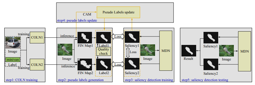
The rapid development of deep learning has made a great progress in salient object detection task. Fully supervised methods need a large number of pixel-level annotations. To avoid laborious and consuming annotation, weakly supervised methods consider low-cost annotations such as category, bounding-box, scribble, etc. Due to simple annotation and existing large-scale classification datasets, the category annotation based methods have received more attention while still suffering from inaccurate detection. In this work, we proposed one weakly supervised method with category annotation. First, we proposed one coarse object location network (COLN) to roughly locate the object of an image with category annotation. Second, we refined the coarse object location to generate pixel-level pseudo-labels and proposed one quality check strategy to select high quality pseudo labels. To this end, we studied COLN twice followed by refinement to obtain a pseudo-labels pair and calculated the consistency of pseudo-label pairs to select high quality labels. Third, we proposed one multi-decoder neural network (MDN) for saliency detection supervised by pseudo-label pairs. The loss of each decoder and between decoders are both considered. Last but not least, we proposed one pseudo-labels update strategy to iteratively optimize pseudo-labels and saliency detection models. Performance evaluation on four public datasets shows that our method outperforms other image category annotation based work.

References

[1]	R. Fan, Q. Hou, M. M. Cheng, G. Yu, R. R. Martin, S. M. Hu, Associating inter-image salient instances for weakly supervised semantic segmentation, in Proceedings of the European Conference on Computer Vision, (2018), 367–383. https://doi.org/10.1007/978-3-030-01240-3_23
[2]	N. Meeboonmak, N. Cooharojananone, Aircraft segmentation from remote sensing images using modified deeply supervised salient object detection with short connections, in International Conference on Mathematics and Computers in Science and Engineering, (2020), 184–187. https://doi.org/10.1109/MACISE49704.2020.00040
[3]	X. Yao, R. Li, J. Zhang, J. Sun, C. Zhang, Explicit boundary guided semi-push-pull contrastive learning for supervised anomaly detection, in Proceedings of the IEEE Conference on Computer Vision and Pattern Recognition, (2023), 24490–24499.
[4]	N. Yu, H. Li, Q. Xu, A full-flow inspection method based on machine vision to detect wafer surface defects, Math. Biosci. Eng., 20 (2023), 11821–11846. https://doi.org/10.3934/mbe.2023526 doi: 10.3934/mbe.2023526
[5]	S. Hong, T. You, S. Kwak, B. Han, Online tracking by learning discriminative saliency map with convolutional neural network, in International Conference on Machine Learning, (2015), 597–606. https://doi.org/10.48550/arXiv.1502.06796
[6]	Q. Yan, L. Xu, J. Shi, J. Jia, Hierarchical saliency detection, in Proceedings of the IEEE Conference on Computer Vision and Pattern Recognition, (2013), 1155–1162. https://doi.org/10.1109/CVPR.2013.153
[7]	F. Perazzi, P. Krähenbühl, Y. Pritch, A. Hornung, Saliency filters: Contrast based filtering for salient region detection, in 2012 IEEE Conference on Computer Vision and Pattern Recognition, (2012), 733–740. https://doi.org/10.1109/CVPR.2012.6247743
[8]	L. Zhang, W. Chen, W. Wang, Z. Jin, C. Zhao, Z. Cai, et al., CBGRU: A detection method of smart contract vulnerability based on a hybrid model, Sensors, 22 (2022), 3577. https://doi.org/10.3390/s22093577 doi: 10.3390/s22093577
[9]	L. Zhang, Y. Li, T. Jin, W. Wang, Z. Jin, C. Zhao, et al., SPCBIG-EC: a robust serial hybrid model for smart contract vulnerability detection, Sensors, 22 (2022), 4621. https://doi.org/10.3390/s22124621 doi: 10.3390/s22124621
[10]	L. Zhang, J. Wang, W. Wang, Z. Jin, C. Zhao, Z. Cai, et al., A novel smart contract vulnerability detection method based on information graph and ensemble learning, Sensors, 22 (2022), 3581, https://doi.org/10.3390/s22093581 doi: 10.3390/s22093581
[11]	K. He, X. Zhang, S. Ren, J. Sun, Deep residual learning for image recognition, in Proceedings of the IEEE Conference on Computer Vision and Pattern Recognition, (2016), 770–778. https://doi.org/10.1109/CVPR.2016.90
[12]	Y. Li, H. Jin, Z. Li, A weakly supervised learning-based segmentation network for dental diseases, Math. Biosci. Eng., 20 (2023), 2039–2060. https://doi.org/10.3934/mbe.2023094 doi: 10.3934/mbe.2023094
[13]	F. Chen, H. Ma, W. Zhang, SegT: Separated edge-guidance transformer network for polyp segmentation, Math. Biosci. Eng., 20 (2023), 17803–17821. https://doi.org/10.3934/mbe.2023791 doi: 10.3934/mbe.2023791
[14]	Q. Feng, X. Xu, Z. Wang, Deep learning-based small object detection: A survey, Math. Biosci. Eng., 20 (2023), 6551–6590. https://doi.org/10.3934/mbe.2023282 doi: 10.3934/mbe.2023282
[15]	C. Wu, L. Chen, A model with deep analysis on a large drug network for drug classification, Math. Biosci. Eng., 20 (2023), 383–401. https://doi.org/10.3934/mbe.2023018 doi: 10.3934/mbe.2023018
[16]	X. Qin, Z. Zhang, C. Huang, C. Gao, M. Dehghan, M. Jagersand, BASNet: Boundary-aware salient object detection, in Proceedings of the IEEE Conference on Computer Vision and Pattern Recognition, (2019), 7479–7489. https://doi.org/10.1109/CVPR.2019.00766
[17]	J. X. Zhao, J. J. Liu, D. P. Fan, Y. Cao, J. Yang, M. M. Cheng, EGNet: Edge guidance network for salient object detection, in Proceedings of the IEEE International Conference on Computer Vision, (2019), 8779–8788. https://doi.org/10.1109/ICCV.2019.00887
[18]	W. Wang, S. Zhao, J. Shen, S. C. Hoi, A. Borji, Salient object detection with pyramid attention and salient edges, in Proceedings of the IEEE Conference on Computer Vision and Pattern Recognition, (2019), 1448–1457. https://doi.org/10.1109/CVPR.2019.00154
[19]	Y. Liu, P. Wang, Y. Cao, Z. Liang, R. W. Lau, Weakly-supervised salient object detection with saliency bounding boxes, IEEE Trans. Image Process., 30 (2021), 4423–4435. https://doi.org/10.1109/TIP.2021.3071691 doi: 10.1109/TIP.2021.3071691
[20]	G. Li, Y. Xie, L. Lin, Weakly supervised salient object detection using image labels, in Proceedings of the AAAI Conference on Artificial Intelligence, 32 (2018), 7024–7031. https://doi.org/10.1609/aaai.v32i1.12308
[21]	Y. Piao, J. Wang, M. Zhang, H. Lu, MFNet: Multi-filter directive network for weakly supervised salient object detection, in Proceedings of the IEEE International Conference on Computer Vision, (2021), 4136–4145. https://doi.org/10.1109/ICCV48922.2021.00410
[22]	Y. Piao, W. Wu, M. Zhang, Y. Jiang, H. Lu, Noise-sensitive adversarial learning for weakly supervised salient object detection, IEEE Trans. Multimedia, 25 (2023), 2888–2897. https://doi.org/10.1109/TMM.2022.3152567 doi: 10.1109/TMM.2022.3152567
[23]	J. Zhang, X. Yu, A. Li, P. Song, B. Liu, Y. Dai, Weakly-supervised salient object detection via scribble annotations, in Proceedings of the IEEE Conference on Computer Vision and Pattern Recognition, (2020), 12546–12555. https://doi.org/10.1109/CVPR42600.2020.01256
[24]	B. Zhou, A. Khosla, A. Lapedriza, A. Oliva, A. Torralba, Learning deep features for discriminative localization, in Proceedings of the IEEE Conference on Computer Vision and Pattern Recognition, (2016), 2921–2929. https://doi.org/10.1109/CVPR.2016.319
[25]	L. Wang, H. Lu, Y. Wang, M. Feng, D. Wang, B. Yin, et al., Learning to detect salient objects with image-level supervision, in Proceedings of the IEEE Conference on Computer Vision and Pattern Recognition, (2017), 136–145. https://doi.org/10.1109/CVPR.2017.404
[26]	X. Zhu, C. Tang, P. Wang, H. Xu, M. Wang, J. Che, et al., Saliency detection via affinity graph learning and weighted manifold ranking, Neurocomputing, 312 (2018), 239–250. https://doi.org/10.1016/j.neucom.2018.05.106 doi: 10.1016/j.neucom.2018.05.106
[27]	W. Zou, N. Komodakis, HARF: Hierarchy-associated rich features for salient object detection, in Proceedings of the IEEE International Conference on Computer Vision, (2015), 406–414. https://doi.org/10.1109/ICCV.2015.54
[28]	Y. Pang, X. Zhao, L. Zhang, H. Lu, Multi-scale interactive network for salient object detection, in Proceedings of the IEEE Conference on Computer Vision and Pattern Recognition, (2020), 9413–9422. https://doi.org/10.1109/CVPR42600.2020.00943
[29]	X. Qin, Z. Zhang, C. Huang, M. Dehghan, O. R. Zaiane, M. Jagersand, U2-Net: Going deeper with nested U-structure for salient object detection, Pattern Recognit., 106 (2020), 107404. https://doi.org/10.1016/j.patcog.2020.107404 doi: 10.1016/j.patcog.2020.107404
[30]	X. Zhao, Y. Pang, L. Zhang, H. Lu, L. Zhang, Suppress and balance: A simple gated network for salient object detection, in Proceedings of the European Conference on Computer Vision, (2020), 35–51. https://doi.org/10.1007/978-3-030-58536-5_3
[31]	L. Tang, B. Li, Y. Zhong, S. Ding, M. Song, Disentangled high quality salient object detection, in Proceedings of the IEEE International Conference on Computer Vision, (2021), 3580–3590. https://doi.org/10.1109/ICCV48922.2021.00356
[32]	M. Ma, C. Xia, J. Li, Pyramidal feature shrinking for salient object detection, in Proceedings of the AAAI Conference on Artificial Intelligence, 35 (2021), 2311–2318. https://doi.org/10.1609/aaai.v35i3.16331
[33]	Y. Song, H. Tang, M. Zhao, N. Sebe, W. Wang, Quasi-equilibrium feature pyramid network for salient object detection, IEEE Trans. Image Process., 31 (2022), 7144–7153. https://doi.org/10.1109/TIP.2022.322005 doi: 10.1109/TIP.2022.322005
[34]	M. Zhuge, D. P. Fan, N. Liu, D. Zhang, D. Xu, L. Shao, Salient object detection via integrity learning, IEEE Trans. Pattern Anal. Mach. Intell., 45 (2022), 3738–3752. https://doi.org/10.1109/TPAMI.2022.3179526 doi: 10.1109/TPAMI.2022.3179526
[35]	Z. Wu, S. Li, C. Chen, H. Qin, A. Hao, Salient object detection via dynamic scale routing, IEEE Trans. Image Process., 31 (2022), 6649–6663. https://doi.org/10.1109/TIP.2022.3214332 doi: 10.1109/TIP.2022.3214332
[36]	Y. H. Wu, Y. Liu, L. Zhang, M. M. Cheng, B. Ren, EDN: Salient object detection via extremely-downsampled network, IEEE Trans. Image Process., 31 (2022), 3125–3136. https://doi.org/10.1109/TIP.2022.3164550 doi: 10.1109/TIP.2022.3164550
[37]	M. Ma, C. Xia, C. Xie, X. Chen, J. Li, Boosting broader receptive fields for salient object detection, IEEE Trans. Image Process., 32 (2023), 1026–1038.https://doi.org/10.1109/TIP.2022.3232209 doi: 10.1109/TIP.2022.3232209
[38]	R. Bi, C. Ji, Z. Yang, M. Qiao, P. Lv, H. Wang, Residual based attention-unet combing DAC and RMP modules for automatic liver tumor segmentation in CT, Math. Biosci. Eng., 19 (2022), 4703–4718. https://doi.org/10.3934/mbe.2022219 doi: 10.3934/mbe.2022219
[39]	H. Zhu, X. He, M. Wang, M. Zhang, L. Qing, Medical visual question answering via corresponding feature fusion combined with semantic attention, Math. Biosci. Eng., 19 (2022), 10192–10212. https://doi.org/10.3934/mbe.2022478 doi: 10.3934/mbe.2022478
[40]	C. Jin, J. Huang, T. Wei, Y. Chen, Neural architecture search based on dual attention mechanism for image classification, Math. Biosci. Eng., 20 (2023), 2691–2715. https://doi.org/10.3934/mbe.2023126 doi: 10.3934/mbe.2023126
[41]	M. Chen, S. Yi, M. Yang, Z. Yang, X. Zhang, Unet segmentation network of COVID-19 CT images with multi-scale attention, Math. Biosci. Eng., 20 (2023), 16762–16785. https://doi.org/10.3934/mbe.2023747 doi: 10.3934/mbe.2023747
[42]	N. Liu, N. Zhang, K. Wan, L. Shao, J. Han, Visual saliency transformer, in Proceedings of the IEEE International Conference on Computer Vision, (2021), 4722–4732. https://doi.org/10.1109/ICCV48922.2021.00468
[43]	Z. Wang, P. Wang, Y. Han, X. Zhang, M. Sun, Q. Tian, Curiosity-driven salient object detection with fragment attention, IEEE Trans. Image Process., 31 (2022), 5989–6001. https://doi.org/10.1109/TIP.2022.3203605 doi: 10.1109/TIP.2022.3203605
[44]	C. Xie, C. Xia, M. Ma, Z. Zhao, X. Chen, J. Li, Pyramid grafting network for one-stage high resolution saliency detection, in Proceedings of the IEEE Conference on Computer Vision and Pattern Recognition, (2022), 11717–11726. https://doi.org/10.1109/CVPR52688.2022.01142
[45]	D. P. Fan, J. Zhang, G. Xu, M. M. Cheng, L. Shao, Salient objects in clutter, IEEE Trans. Pattern Anal. Mach. Intell., 45 (2022), 2344–2366. https://doi.org/10.1109/TPAMI.2022.3166451
[46]	M. M. Cheng, S. H. Gao, A. Borji, Y. Q. Tan, Z. Lin, M. Wang, A highly efficient model to study the semantics of salient object detection, IEEE Trans. Pattern Anal. Mach. Intell., 44 (2021), 8006–8021. https://doi.org/110.1109/TPAMI.2021.3107956
[47]	X. Tian, K. Xu, X. Yang, L. Du, B. Yin, R. W. Lau, Bi-directional object-context prioritization learning for saliency ranking, in Proceedings of the IEEE/CVF Conference on Computer Vision and Pattern Recognition, (2022), 5882–5891.
[48]	X. Tian, X. Yang, B. Yin, R. W. Lau, Weakly-supervised salient instance detection, preprint, arXiv: 2009.13898.
[49]	X. Tian, K. Xu, X. Yang, B. Yin, R. W. Lau, Learning to detect instance-level salient objects using complementary image labels, Int. J. Comput. Vision, 130 (2022), 729–746. https://doi.org/10.1007/s11263-021-01553-w doi: 10.1007/s11263-021-01553-w
[50]	Z. Liang, P. Wang, K. Xu, P. Zhang, R. W. Lau, Weakly-supervised salient object detection on light fields, IEEE Trans. Image Process., 31 (2022), 6295–6305. https://doi.org/10.1109/TIP.2022.3207605 doi: 10.1109/TIP.2022.3207605
[51]	X. Zheng, X. Tan, J. Zhou, L. Ma, R. W. H. Lau, Weakly-supervised saliency detection via salient object subitizing, IEEE Trans. Circuits Syst. Video Technol., 31 (2021), 4370–4380. https://doi.org/10.1109/TCSVT.2021.3049408 doi: 10.1109/TCSVT.2021.3049408
[52]	X. Liu, J. Guo, S. Zheng, Weakly-supervised salient object detection with label decoupling siamese network, in Proceedings of the 8th International Conference on Computing and Artificial Intelligence, (2022), 412–418. https://doi.org/10.1145/3532213.3532275
[53]	Y. Zeng, Y. Zhuge, H. Lu, L. Zhang, M. Qian, Y. Yu, Multi-source weak supervision for saliency detection, in Proceedings of the IEEE Conference on Computer Vision and Pattern Recognition, (2019), 6074–6083. https://doi.org/10.1109/CVPR.2019.00623
[54]	H. Zhang, Y. Zeng, H. Lu, L. Zhang, J. Li, J. Qi, Learning to detect salient object with multi-source weak supervision, IEEE Trans. Pattern Anal. Mach. Intell., 44 (2021), 3577–3589. https://doi.org/10.1109/TPAMI.2021.3059783 doi: 10.1109/TPAMI.2021.3059783
[55]	C. Rother, GrabCut: interactive foreground extraction using iterated graph cuts, ACM Trans. Graphics, 23 (2004), 309–314. https://doi.org/10.1145/1015706.1015720 doi: 10.1145/1015706.1015720
[56]	Y. Boykov, M. Jolly, Interactive graph cuts for optimal boundary and region segmentation of objects in n-d images, in Proceedings of the IEEE International Conference on Computer Vision, (2001), 105–112. https://doi.org/10.1109/ICCV.2001.937505
[57]	J. J. Liu, Q. Hou, M. M. Cheng, J. Feng, J. Jiang, A simple pooling-based design for real-time salient object detection, in Proceedings of the IEEE Conference on Computer Vision and Pattern Recognition, (2019), 3917–3926. https://doi.org/10.1109/CVPR.2019.00404
[58]	K. Simonyan, A. Zisserman, Very deep convolutional networks for large-scale image recognition, preprint, arXiv: 1409.1556.
[59]	Y. Li, X. Hou, C. Koch, J. M. Rehg, A. L. Yuille, The secrets of salient object segmentation, in Proceedings of the IEEE Conference on Computer Vision and Pattern Recognition, (2014), 280–287. https://doi.org/10.1109/CVPR.2014.43
[60]	G. Li, Y. Yu, Visual saliency based on multiscale deep features, in Proceedings of the IEEE Conference on Computer Vision and Pattern Recognition, (2015), 5455–5463. https://doi.org/10.1109/CVPR.2015.7299184
[61]	Y. Liu, X. Y. Zhang, J. W. Bian, L. Zhang, M. M. Cheng, SAMNet: Stereoscopically attentive multi-scale network for lightweight salient object detection, IEEE Trans. Image Process., 30 (2021), 3804–3814. https://doi.org/10.1109/TIP.2021.3065239 doi: 10.1109/TIP.2021.3065239
[62]	X. Zhang, T. Wang, J. Qi, H. Lu, G. Wang, Progressive attention guided recurrent network for salient object detection, in Proceedings of the IEEE Conference on Computer Vision and Pattern Recognition, (2018), 714–722.
[63]	T. Zhao, X. Wu, Pyramid feature attention network for saliency detection, in Proceedings of the IEEE/CVF Conference on Computer Vision and Pattern Recognition, (2019), 3085–3094.
[64]	P. Zhang, D. Wang, H. Lu, H. Wang, B. Yin, Learning uncertain convolutional features for accurate saliency detection, in Proceedings of the IEEE International Conference on Computer Vision, (2017), 212–221.

Reader Comments

Your name:*

Email:*
© 2023 the Author(s), licensee AIMS Press. This is an open access article distributed under the terms of the Creative Commons Attribution License (http://creativecommons.org/licenses/by/4.0)