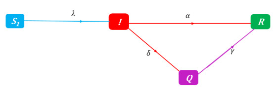
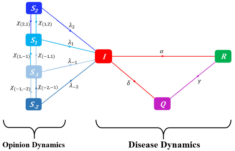
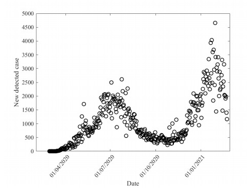
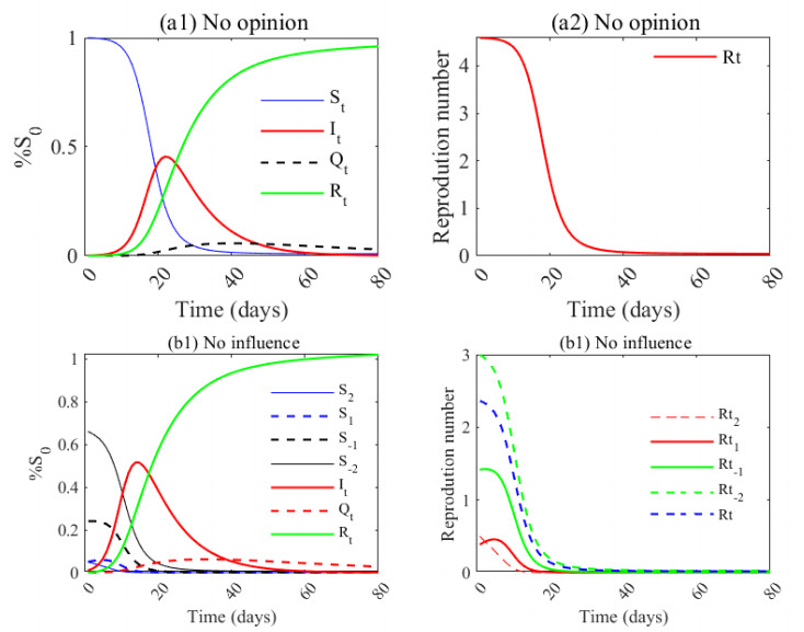
Various general and individual measures have been implemented to limit the spread of SARS-CoV-2 since its emergence in China. Several phenomenological and mechanistic models have been developed to inform and guide health policy. Many of these models ignore opinions about certain control measures, although various opinions and attitudes can influence individual actions. To account for the effects of prophylactic opinions on disease dynamics and to avoid identifiability problems, we expand the SIR-Opinion model of Tyson et al. (2020) to take into account the partial detection of infected individuals in order to provide robust modeling of COVID-19 as well as degrees of adherence to prophylactic treatments, taking into account a hybrid modeling technique using Richard's model and the logistic model. Applying the approach to COVID-19 data from West Africa demonstrates that the more people with a strong prophylactic opinion, the smaller the final COVID-19 pandemic size. The influence of individuals on each other and from the media significantly influences the susceptible population and, thus, the dynamics of the disease. Thus, when considering the opinion of susceptible individuals to the disease, the view of the population at baseline influences its dynamics. The results are expected to inform public policy in the context of emerging and re-emerging infectious diseases.
Citation: Elodie Yedomonhan, Chénangnon Frédéric Tovissodé, Romain Glèlè Kakaï. Modeling the effects of Prophylactic behaviors on the spread of SARS-CoV-2 in West Africa[J]. Mathematical Biosciences and Engineering, 2023, 20(7): 12955-12989. doi: 10.3934/mbe.2023578
Various general and individual measures have been implemented to limit the spread of SARS-CoV-2 since its emergence in China. Several phenomenological and mechanistic models have been developed to inform and guide health policy. Many of these models ignore opinions about certain control measures, although various opinions and attitudes can influence individual actions. To account for the effects of prophylactic opinions on disease dynamics and to avoid identifiability problems, we expand the SIR-Opinion model of Tyson et al. (2020) to take into account the partial detection of infected individuals in order to provide robust modeling of COVID-19 as well as degrees of adherence to prophylactic treatments, taking into account a hybrid modeling technique using Richard's model and the logistic model. Applying the approach to COVID-19 data from West Africa demonstrates that the more people with a strong prophylactic opinion, the smaller the final COVID-19 pandemic size. The influence of individuals on each other and from the media significantly influences the susceptible population and, thus, the dynamics of the disease. Thus, when considering the opinion of susceptible individuals to the disease, the view of the population at baseline influences its dynamics. The results are expected to inform public policy in the context of emerging and re-emerging infectious diseases.

| [1] | S. Dasgupta, R. Crunkhorn, A History of pandemics over the ages and the human cost, The Physician, 6 (2020). https://doi.org/10.38192/1.6.2.1 |
| [2] | W. Byrd, M. Salcher-Konrad, S. Smith, A. Comas-Herrera, What long-term care interventions and policy measures have been studied during the covid-19 pandemic? findings from a rapid mapping review of the scientific evidence published during 2020, J. Long-Term Care, (2020), 423–437. https://doi.org/10.31389/jltc.97 |
| [3] |
D. Khan, N. Ahmed, B. Mehmed, I. u. Haq, Assessing the Impact of Policy Measures in Reducing the COVID-19 Pandemic: A Case Study of South Asia, Sustainability, 13 (2021), 11315. https://doi.org/10.3390/su132011315 doi: 10.3390/su132011315

|
| [4] |
N. Perra, Non-pharmaceutical interventions during the COVID-19 pandemic: A review, Phys. Rep., 913 (2021), 1–52. https://doi.org/10.3390/s22010280 doi: 10.3390/s22010280
|
| [5] |
I. Sabat, S. Neumann-Böhme, N. E. Varghese, P. P. Barros, W. Brouwer, J. van Exel, et al., United but divided: Policy responses and people's perceptions in the EU during the COVID-19 outbreak, Health Policy, 124 (2020), 909–918. https://doi.org/10.1016/j.healthpol.2020.06.009 doi: 10.1016/j.healthpol.2020.06.009
|
| [6] |
S. Talic, S. Shah, H. Wild, D. Gasevic, A. Maharaj, Z. Ademi, et al., Effectiveness of public health measures in reducing the incidence of covid-19, sars-cov-2 transmission, and covid-19 mortality: Systematic review and meta-analysis, BMJ, 375 (2021), e068302. https://doi.org/10.1136/bmj-2021-068302 doi: 10.1136/bmj-2021-068302
|
| [7] |
P. Deb, D. Furceri, J. D. Ostry, N. Tawk, The economic effects of covid-19 containment measures, Open Econ. Rev., 33 (2022), 1–32. https://doi.org/10.1007/s11079-021-09638-2 doi: 10.1007/s11079-021-09638-2
|
| [8] |
W. Ahmad, K. Shabbiri, Two years of sars-cov-2 infection (2019–2021): Structural biology, vaccination, and current global situation, Egyptian J. Int. Med., 34 (2022), 1–12. https://doi.org/10.1186/s43162-021-00092-7 doi: 10.1186/s43162-021-00092-7
|
| [9] |
K. Tao, P. L. Tzou, J. Nouhin, R. K. Gupta, T. de Oliveira, S. L. Kosakovsky Pond, et al., The biological and clinical significance of emerging SARS-CoV-2 variants, Nat. Rev. Genet., 22 (2021), 757–773. https://doi.org/10.1038/s41576-021-00408-x doi: 10.1038/s41576-021-00408-x
|
| [10] | F. Wu, R. Yan, M. Liu, Z. Liu, Y. Wang, D. Luan, et al., Antibody-dependent enhancement (ade) of sars-cov-2 infection in recovered covid-19 patients: Studies based on cellular and structural biology analysis, MedRxiv. https://doi.org/10.1101/2020.10.08.20209114 |
| [11] | W. Yan, Y. Zheng, X. Zeng, B. He, W. Cheng, Structural biology of SARS-CoV-2: Open the door for novel therapies, Signal Transduct. Targeted Therapy, 7 (2022), 1–28. https://www.nature.com/articles/s41392-022-00884-5 |
| [12] |
H. Yang, Z. Rao, Structural biology of SARS-CoV-2 and implications for therapeutic development, Nat. Rev. Microbiol., 19 (2021), 685–700. https://doi.org/10.1038/s41579-021-00630-8 doi: 10.1038/s41579-021-00630-8
|
| [13] | Y. Wu, J. Liu, M. Liu, Evaluation of COVID-19 outbreak prevention and control in Beijing using the emergency management theory, Fundament. Res., (2022). https://doi.org/10.1016/j.fmre.2022.06.005 |
| [14] |
B. Yuan, R. Liu, S. Tang, A quantitative method to project the probability of the end of an epidemic: Application to the COVID-19 outbreak in Wuhan, 2020, J. Theoret. Biol., 545 (2022), 111149. https://doi.org/10.1016/j.jtbi.2022.111149 doi: 10.1016/j.jtbi.2022.111149
|
| [15] |
C. Yang, S. Zhang, S. Lu, J. Yang, Y. Cheng, Y. Liu, et al., All five COVID-19 outbreaks during epidemic period of 2020/2021 in China were instigated by asymptomatic or pre-symptomatic individuals, J. Biosafety Biosecur., 3 (2021), 35–40. https://doi.org/10.1016/j.jobb.2021.04.001 doi: 10.1016/j.jobb.2021.04.001
|
| [16] | M. J. Ali, A. B. Bhuiyan, N. Zulkifli, M. K. Hassan, The COVID-19 Pandemic: Conceptual Framework for the Global Economic Impacts and Recovery, in Towards a Post-Covid Global Financial System (eds. M. Kabir Hassan, A. Muneeza and A. M. Sarea), Emerald Publishing Limited, 2022,225–242. https://doi.org/10.1108/978-1-80071-625-420210012 |
| [17] |
I. Chakraborty, P. Maity, COVID-19 outbreak: Migration, effects on society, global environment and prevention, Sci. Total Environ., 728 (2020), 138882. https://doi.org/10.1016/j.scitotenv.2020.138882 doi: 10.1016/j.scitotenv.2020.138882
|
| [18] |
A. Facciolà, P. Laganà, G. Caruso, The COVID-19 pandemic and its implications on the environment, Environmental Research, 201 (2021), 111648. https://doi.org/10.3389/fpubh.2020.00241 doi: 10.3389/fpubh.2020.00241
|
| [19] | A. Pak, O. A. Adegboye, A. I. Adekunle, K. M. Rahman, E. S. McBryde, D. P. Eisen, Economic Consequences of the COVID-19 Outbreak: The Need for Epidemic Preparedness, Front. Public Health, 8 (2020). https://doi.org/10.3389/fpubh.2020.00241 |
| [20] |
C. F. Tovissodé, J. T. Doumatè, R. Glèlè Kakaï, A Hybrid Modeling Technique of Epidemic Outbreaks with Application to COVID-19 Dynamics in West Africa, Biology, 10 (2021), 365. https://doi.org/10.3390/biology10050365 doi: 10.3390/biology10050365
|
| [21] |
J. E. Gnanvi, K. V. Salako, G. B. Kotanmi, R. Glèlè Kakaï, On the reliability of predictions on Covid-19 dynamics: A systematic and critical review of modelling techniques, Infect. Disease Model., 6 (2021), 258–272. https://doi.org/10.1016/j.idm.2020.12.008 doi: 10.1016/j.idm.2020.12.008
|
| [22] |
C. Giambiagi Ferrari, J. P. Pinasco, N. Saintier, Coupling Epidemiological Models with Social Dynamics, Bull. Math. Biol., 83 (2021), 74. https://doi.org/10.1007/s11538-021-00910-7 doi: 10.1007/s11538-021-00910-7
|
| [23] | R. Prieto Curiel, H. González Ramírez, Vaccination strategies against COVID-19 and the diffusion of anti-vaccination views, Sci. Rep., 11 (2021), 1–13. https://www.nature.com/articles/s41598-021-85555-1 |
| [24] |
J. Sooknanan, D. M. G. Comissiong, Trending on Social Media: Integrating Social Media into Infectious Disease Dynamics, Bull. Math. Biol., 82 (2020), 86. https://doi.org/10.1007/s11538-020-00757-4 doi: 10.1007/s11538-020-00757-4
|
| [25] |
P. C. V. da Silva, F. Velásquez-Rojas, C. Connaughton, F. Vazquez, Y. Moreno, F. A. Rodrigues, Epidemic spreading with awareness and different timescales in multiplex networks, Phys. Rev. E, 100 (2019), 032313. https://doi.org/10.1103/PhysRevE.100.032313 doi: 10.1103/PhysRevE.100.032313
|
| [26] |
Y. Zhou, J. Zhou, G. Chen, H. E. Stanley, Effective degree theory for awareness and epidemic spreading on multiplex networks, New J. Phys., 21 (2019), 035002. https://doi.org/10.1088/1367-2630/ab0458 doi: 10.1088/1367-2630/ab0458
|
| [27] |
G. O. Agaba, Y. N. Kyrychko, K. B. Blyuss, Mathematical model for the impact of awareness on the dynamics of infectious diseases, Math. Biosci., 286 (2017), 22–30. https://doi.org/10.1016/j.mbs.2017.01.009 doi: 10.1016/j.mbs.2017.01.009
|
| [28] |
M. A. Pires, N. Crokidakis, Dynamics of epidemic spreading with vaccination: Impact of social pressure and engagement, Phys. A Stat. Mech. Appl., 467 (2017), 167–179. https://doi.org/10.1016/j.physa.2016.10.004 doi: 10.1016/j.physa.2016.10.004
|
| [29] |
F. Verelst, L. Willem, P. Beutels, Behavioural change models for infectious disease transmission: a systematic review (2010–2015), J. Royal Soc. Interf., 13 (2016), 20160820. https://doi.org/10.1098/rsif.2016.0820 doi: 10.1098/rsif.2016.0820
|
| [30] |
E. P. Fenichel, C. Castillo-Chavez, M. G. Ceddia, G. Chowell, P. A. G. Parra, G. J. Hickling, et al., Adaptive human behavior in epidemiological models, Proceed. Nat. Aca. Sci., 108 (2011), 6306–6311. https://doi.org/10.1073/pnas.1011250108 doi: 10.1073/pnas.1011250108
|
| [31] |
S. Funk, M. Salathé, V. A. A. Jansen, Modelling the influence of human behaviour on the spread of infectious diseases: A review, J. Royal Soc. Interf., 7 (2010), 1247–1256. https://doi.org/10.1098/rsif.2010.0142 doi: 10.1098/rsif.2010.0142
|
| [32] |
S. Bansal, B. T. Grenfell, L. A. Meyers, When individual behaviour matters: homogeneous and network models in epidemiology, J. Royal Soc. Interf., 4 (2007), 879–891. https://doi.org/10.1098/rsif.2007.1100 doi: 10.1098/rsif.2007.1100
|
| [33] | S. S. Musa, W. Xueying, Z. Shi, L. Shudong, H. Nafiu, W. Weiming et al., The heterogeneous severity of covid-19 in african countries: A modeling approach, Bull. Math. Biol., 84 (2022). https://doi.org/10.1007/s11538-022-00992-x |
| [34] |
R. C. Tyson, S. D. Hamilton, A. S. Lo, B. O. Baumgaertner, S. M. Krone, The Timing and Nature of Behavioural Responses Affect the Course of an Epidemic, Bull. Math. Biol., 82 (2020), 14. https://doi.org/10.1007/s11538-019-00684-z doi: 10.1007/s11538-019-00684-z
|
| [35] |
M. K. Kanadiya, A. M. Sallar, Preventive behaviors, beliefs, and anxieties in relation to the swine flu outbreak among college students aged 18–24 years, J. Public Health, 19 (2011), 139–145. https://doi.org/10.1007/s10389-010-0373-3 doi: 10.1007/s10389-010-0373-3
|
| [36] |
I. C.-H. Fung, S. Cairncross, How often do you wash your hands? A review of studies of hand-washing practices in the community during and after the SARS outbreak in 2003, Int. J. Environ. Health Res., 17 (2007), 161–183. https://doi.org/10.1080/09603120701254276 doi: 10.1080/09603120701254276
|
| [37] |
M. Z. Sadique, W. J. Edmunds, R. D. Smith, W. J. Meerding, O. de Zwart, J. Brug, et al., Precautionary Behavior in Response to Perceived Threat of Pandemic Influenza, Emerg. Infect. Diseases, 13 (2007), 1307–1313. https://doi.org/10.3201/eid1309.070372 doi: 10.3201/eid1309.070372
|
| [38] |
J. T. Lau, X. Yang, E. Pang, H. Tsui, E. Wong, Y. K. Wing, SARS-related Perceptions in Hong Kong, Emerg. Infect. Diseases, 11 (2005), 417–424. https://doi.org/10.3201/eid1103.040675 doi: 10.3201/eid1103.040675
|
| [39] |
B. Rosen, R. Waitzberg, A. Israeli, M. Hartal, N. Davidovitch, Addressing vaccine hesitancy and access barriers to achieve persistent progress in israel's covid-19 vaccination program, Israel J. Health Pol. Res., 10 (2021), 1–20. https://doi.org/10.1186/s13584-021-00481-x doi: 10.1186/s13584-021-00481-x
|
| [40] |
G. Akdeniz, M. Kavakci, M. Gozugok, S. Yalcinkaya, A. Kucukay, B. Sahutogullari, A survey of attitudes, anxiety status, and protective behaviors of the university students during the covid-19 outbreak in turkey, Front. Psych., 11 (2020), 695. https://doi.org/10.3389/fpsyt.2020.00695 doi: 10.3389/fpsyt.2020.00695
|
| [41] |
S. F. Costa, S. Vernal, P. Giavina-Bianchi, C. H. Mesquita Peres, L. G. D. dos Santos, R. E. B. Santos, et al., Adherence to non-pharmacological preventive measures among healthcare workers in a middle-income country during the first year of the COVID-19 pandemic: Hospital and community setting, Am. J. Infect. Control, 50 (2022), 707–711. https://doi.org/10.1016/j.ajic.2021.12.004 doi: 10.1016/j.ajic.2021.12.004
|
| [42] |
A. P. Yan, K. Howden, A. L. Mahar, C. Glidden, S. N. Garland, S. Oberoi, Gender differences in adherence to COVID-19 preventative measures and preferred sources of COVID-19 information among adolescents and young adults with cancer, Cancer Epidemiol., 77 (2022), 102098. https://doi.org/10.1016/j.canep.2022.102098 doi: 10.1016/j.canep.2022.102098
|
| [43] |
R. A. Elhameed Ali, A. A. Ghaleb, S. A. Abokresha, Covid-19 Related Knowledge and Practice and Barriers that Hinder Adherence to Preventive Measures among the Egyptian Community. An Epidemiological Study in Upper Egypt, J. Public Health Res., 10 (2021), 1943. https://doi.org/10.4081/jphr.2020.1943 doi: 10.4081/jphr.2020.1943
|
| [44] |
P. G. Devereux, M. K. Miller, J. M. Kirshenbaum, Moral disengagement, locus of control, and belief in a just world: Individual differences relate to adherence to COVID-19 guidelines, Personal. Individual Differ., 182 (2021), 111069. https://doi.org/10.1016/j.paid.2021.111069 doi: 10.1016/j.paid.2021.111069
|
| [45] |
A. Bante, A. Mersha, A. Tesfaye, B. Tsegaye, S. Shibiru, G. Ayele, et al., Adherence with COVID-19 Preventive Measures and Associated Factors Among Residents of Dirashe District, Southern Ethiopia, Patient Prefer. Adher., 15 (2021), 237–249. https://doi.org/10.1371/journal.pone.0275320 doi: 10.1371/journal.pone.0275320
|
| [46] |
T. Varol, R. Crutzen, F. Schneider, I. Mesters, R. A. C. Ruiter, G. Kok, et al., Selection of determinants of students' adherence to COVID-19 guidelines and translation into a brief intervention, Acta Psychol., 219 (2021), 103400. https://doi.org/10.1016/j.actpsy.2021.103400 doi: 10.1016/j.actpsy.2021.103400
|
| [47] |
S. S. Yehualashet, K. K. Asefa, A. G. Mekonnen, B. N. Gemeda, W. S. Shiferaw, Y. A. Aynalem, et al., Predictors of adherence to COVID-19 prevention measure among communities in North Shoa Zone, Ethiopia based on health belief model: A cross-sectional study, PLoS One, 16 (2021), e0246006, https://doi.org/10.1371/journal.pone.0246006 doi: 10.1371/journal.pone.0246006
|
| [48] |
M. Beeckman, A. De Paepe, M. Van Alboom, S. Maes, A. Wauters, F. Baert, et al., Adherence to the Physical Distancing Measures during the COVID-19 Pandemic: A HAPA-Based Perspective, Appl. Psychol. Health Well-Being, 12 (2020), 1224–1243. https://doi.org/10.1111/aphw.12242 doi: 10.1111/aphw.12242
|
| [49] |
A. Coroiu, C. Moran, T. Campbell, A. C. Geller, Barriers and facilitators of adherence to social distancing recommendations during COVID-19 among a large international sample of adults, PLoS One, 15 (2020), e0239795. https://doi.org/10.1371/journal.pone.0239795 doi: 10.1371/journal.pone.0239795
|
| [50] |
K. K. Tong, J. H. Chen, E. W.-y. Yu, A. M. S. Wu, Adherence to COVID-19 Precautionary Measures: Applying the Health Belief Model and Generalised Social Beliefs to a Probability Community Sample, Appl. Psychol. Health Well-Being, 12 (2020), 1205–1223. https://doi.org/10.1111/aphw.12230 doi: 10.1111/aphw.12230
|
| [51] |
T. Xiao, T. Mu, S. Shen, Y. Song, S. Yang, J. He, A dynamic physical-distancing model to evaluate spatial measures for prevention of Covid-19 spread, Physica A: Statistical Mechanics and its Applications, 592 (2022), 126734. https://doi.org/10.1016/j.physa.2021.126734 doi: 10.1016/j.physa.2021.126734
|
| [52] |
O. Agossou, M. N. Atchadé, A. M. Djibril, Modeling the effects of preventive measures and vaccination on the COVID-19 spread in Benin Republic with optimal control, Results Phys., 31 (2021), 104969. https://doi.org/10.1016/j.rinp.2021.104969 doi: 10.1016/j.rinp.2021.104969
|
| [53] |
M. Dashtbali, M. Mirzaie, A compartmental model that predicts the effect of social distancing and vaccination on controlling COVID-19, Sci. Rep., 11 (2021), 8191. https://doi.org/10.1038/s41598-021-86873-0 doi: 10.1038/s41598-021-86873-0
|
| [54] |
R. Prabakaran, S. Jemimah, P. Rawat, D. Sharma, M. M. Gromiha, A novel hybrid SEIQR model incorporating the effect of quarantine and lockdown regulations for COVID-19, Sci. Rep., 11 (2021), 24073. https://doi.org/10.1038/s41598-021-03436-z doi: 10.1038/s41598-021-03436-z
|
| [55] |
Z. Zhang, L. Kong, H. Lin, G. Zhu, Modeling coupling dynamics between the transmission, intervention of COVID-19 and economic development, Results Phys., 28 (2021), 104632. https://doi.org/10.1016/j.rinp.2021.104632 doi: 10.1016/j.rinp.2021.104632
|
| [56] |
W. C. Koh, L. Naing, J. Wong, Estimating the impact of physical distancing measures in containing COVID-19: an empirical analysis, Int. J. Infect. Diseases, 100 (2020), 42–49. https://doi.org/10.1016/j.ijid.2020.08.026 doi: 10.1016/j.ijid.2020.08.026
|
| [57] |
S. Mwalili, M. Kimathi, V. Ojiambo, D. Gathungu, R. Mbogo, SEIR model for COVID-19 dynamics incorporating the environment and social distancing, BMC Res. Notes, 13 (2020), 352. https://doi.org/10.1186/s13104-020-05192-1 doi: 10.1186/s13104-020-05192-1
|
| [58] |
H. B. Taboe, K. V. Salako, J. M. Tison, C. N. Ngonghala, R. G. Kakaï, Predicting COVID-19 spread in the face of control measures in West Africa, Math. Biosci., 328 (2020), 108431. https://doi.org/10.1016/j.mbs.2020.108431 doi: 10.1016/j.mbs.2020.108431
|
| [59] |
S. Wurtzer, V. Marechal, J. M. Mouchel, Y. Maday, R. Teyssou, E. Richard, et al., Evaluation of lockdown effect on SARS-CoV-2 dynamics through viral genome quantification in waste water, Greater Paris, France, 5 March to 23 April 2020, Eurosurveillance, 25 (2020), 2000776. https://doi.org/10.2807/1560-7917.ES.2020.25.50.2000776 doi: 10.2807/1560-7917.ES.2020.25.50.2000776
|
| [60] | B. She, J. Liu, S. Sundaram, P. E. Pare, On a Networked SIS Epidemic Model with Cooperative and Antagonistic Opinion Dynamics, IEEE Transactions on Control of Network Systems, 1. |
| [61] | K. M. Bubar, K. Reinholt, S. M. Kissler, M. Lipsitch, S. Cobey, Y. H. Grad, et al., Model-informed COVID-19 vaccine prioritization strategies by age and serostatus, Science, 371 (2021), 916–921. https://www.science.org/doi/10.1126/science.abe6959 |
| [62] |
W. Xuan, R. Ren, P. E. Paré, M. Ye, S. Ruf, J. Liu, On a Network SIS Model with Opinion Dynamics, IFAC-PapersOnLine, 53 (2020), 2582–2587. https://doi.org/10.1016/j.ifacol.2020.12.305 doi: 10.1016/j.ifacol.2020.12.305
|
| [63] |
K. Liu, Y. Lou, Optimizing COVID-19 vaccination programs during vaccine shortages, Infect. Disease Model., 7 (2022), 286–298. https://doi.org/10.1016/j.idm.2022.02.002 doi: 10.1016/j.idm.2022.02.002
|
| [64] |
E. P. Esteban, L. Almodovar-Abreu, Assessing the impact of vaccination in a COVID-19 compartmental model, Inform. Med. Unlocked, 27 (2021), 100795. https://doi.org/10.1016/j.imu.2021.100795 doi: 10.1016/j.imu.2021.100795
|
| [65] |
E. A. Iboi, C. N. Ngonghala, A. B. Gumel, Will an imperfect vaccine curtail the COVID-19 pandemic in the U.S.?, Infect. Disease Model., 5 (2020), 510–524. https://doi.org/10.1016/j.idm.2020.07.006 doi: 10.1016/j.idm.2020.07.006
|
| [66] |
R. Jankowski, A. Chmiel, Role of Time Scales in the Coupled Epidemic-Opinion Dynamics on Multiplex Networks, Entropy, 24 (2022), 105. https://doi.org/10.3390/e24010105 doi: 10.3390/e24010105
|
| [67] |
Y. Zhang, N. Chen, W. Du, S. Yao, X. Zheng, A New Geo-Propagation Model of Event Evolution Chain Based on Public Opinion and Epidemic Coupling, Int. J. Environm. Res. Public Health, 17 (2020), 9235. https://doi.org/10.3390/ijerph17249235 doi: 10.3390/ijerph17249235
|
| [68] |
Y. Ye, Q. Zhang, Z. Ruan, Z. Cao, Q. Xuan, D. D. Zeng, Effect of heterogeneous risk perception on information diffusion, behavior change, and disease transmission, Phys. Rev. E, 102 (2020), 042314. https://doi.org/10.1103/PhysRevE.102.042314 doi: 10.1103/PhysRevE.102.042314
|
| [69] |
M. Li, R.-R. Liu, D. Peng, C.-X. Jia, B.-H. Wang, Roles of the spreading scope and effectiveness in spreading dynamics on multiplex networks, Phys. A Statist. Mechan. Appl., 492 (2018), 1239–1246. https://doi.org/10.1016/j.physa.2017.11.051 doi: 10.1016/j.physa.2017.11.051
|
| [70] |
M. A. Almadhi, A. Abdulrahman, S. A. Sharaf, D. AlSaad, N. J. Stevenson, S. L. Atkin, et al., The high prevalence of asymptomatic SARS-CoV-2 infection reveals the silent spread of COVID-19, Int. J. Infect. Diseases, 105 (2021), 656–661. https://doi.org/10.1016/j.ijid.2021.02.100 doi: 10.1016/j.ijid.2021.02.100
|
| [71] |
D. P. Oran, E. J. Topol, Prevalence of Asymptomatic SARS-CoV-2 Infection, Ann. Int. Med., 173 (2020), 362–367. https://doi.org/10.7326/M20-3012 doi: 10.7326/M20-3012
|
| [72] |
D. P. Oran, E. J. Topol, The Proportion of SARS-CoV-2 Infections That Are Asymptomatic, Ann. Int. Med., 174 (2021), 655–662. https://doi.org/10.7326/M20-6976 doi: 10.7326/M20-6976
|
| [73] |
H. Hethcote, M. Zhien, L. Shengbing, Effects of quarantine in six endemic models for infectious diseases, Math. Biosci., 180 (2002), 141–160. https://doi.org/10.1016/S0025-5564(02)00111-6 doi: 10.1016/S0025-5564(02)00111-6
|
| [74] |
C. F. Tovissodé, B. E. Lokonon, R. G. Kakaï, On the use of growth models to understand epidemic outbreaks with application to COVID-19 data, PLoS One, 15 (2020), e0240578. https://doi.org/10.1371/journal.pone.0240578 doi: 10.1371/journal.pone.0240578
|
| [75] |
G. Chowell, C. Viboud, L. Simonsen, S. Merler, A. Vespignani, Perspectives on model forecasts of the 2014–2015 Ebola epidemic in West Africa: Lessons and the way forward, BMC Med., 15 (2017), 42. https://doi.org/10.1186/s12916-017-0811-y doi: 10.1186/s12916-017-0811-y
|
| [76] | Y.-H. Hsieh, Richards Model: A Simple Procedure for Real-time Prediction of Outbreak Severity, in Modeling and Dynamics of Infectious Diseases, vol. Volume 11 of Series in Contemporary Applied Mathematics, CO-PUBLISHED WITH HIGHER EDUCATION PRESS, 2009,216–236. https://doi.org/10.1142/9789814261265_0009 |
| [77] |
G. Zhou, G. Yan, Severe acute respiratory syndrome epidemic in Asia., Emerg. Infect. Diseases, 9 (2003), 1608–1610. https://doi.org/10.3201/eid0912.030382 doi: 10.3201/eid0912.030382
|
| [78] |
O. Diekmann, J. Heesterbeek, M. G. Roberts, The construction of next-generation matrices for compartmental epidemic models, J. Royal Soc. Interf., 7 (2010), 873–885. https://doi.org/10.1098/rsif.2009.0386 doi: 10.1098/rsif.2009.0386
|
| [79] |
S. H. Honfo, H. B. Taboe, R. Glèlè Kakaï, Modeling covid-19 dynamics in the sixteen west African countries, Sci. African, 12 (2022), e01408. https://doi.org/10.1016/j.sciaf.2022.e01408 doi: 10.1016/j.sciaf.2022.e01408
|
| [80] | E. Dong, H. Du, L. Gardner, An interactive web-based dashboard to track covid-19 in real time, Lancet Infect. Diseases, 20 (2020), 533–534. |
| [81] |
J. M. Clarke, A. Majeed, T. Beaney, Measuring the impact of covid-19, BMJ, 373 (2021), n1239. https://doi.org/10.1136/bmj.n1239 doi: 10.1136/bmj.n1239
|
| [82] | R Core Team, R: A Language and Environment for Statistical Computing, R Foundation for Statistical Computing, Vienna, Austria, 2020. https://www.R-project.org/ |
| [83] | PERC, La riposte à la covid-19 en afrique: Trouver un équilibre. partie iv, 2022. |
| [84] | T. Miyama, S.-M. Jung, K. Hayashi, A. Anzai, R. Kinoshita, T. Kobayashi, et al., Phenomenological and mechanistic models for predicting early transmission data of covid-19, Math. Biosci. Eng., 19 (2021), 2043–2055. http://www.aimspress.com/article/doi/10.3934/mbe.2022096 |
| [85] |
M. Coccia, hThe impact of first and second wave of the COVID-19 pandemic in society: comparative analysis to support control measures to cope with negative effects of future infectious diseases, Environ. Res., 197 (2021), 111099. https://doi.org/10.1016/j.envres.2021.111099 doi: 10.1016/j.envres.2021.111099
|
| [86] |
E. Du, E. Chen, J. Liu, C. Zheng, How do social media and individual behaviors affect epidemic transmission and control?, Sci. Total Environ., 761 (2021), 144114. https://doi.org/10.1016/j.scitotenv.2020.144114 doi: 10.1016/j.scitotenv.2020.144114
|
| [87] | D. Centola, The spread of behavior in an online social network experiment, Science, 329 (2010), 1194–1197. https://www.science.org/doi/abs/10.1126/science.1185231 |
| [88] |
S. Zhao, G. D. Lewi Stone, S. S. Musa, M. K. C. Chong, D. He, M. H. Wang, Imitation dynamics in the mitigation of the novel coronavirus disease (covid-19) outbreak in wuhan, china from 2019 to 2020, Ann. Transl. Med., 8 (2020), 1–14. doi: 10.21037/atm.2020.03.168 doi: 10.21037/atm.2020.03.168
|
| [89] |
Q. Lin, Z. Shi, G. Daozhou, L. Yijun, Y. Shu, M. Salihu Sabiu, et al., A conceptual model for the coronavirus disease 2019 (covid-19) outbreak in wuhan, china with individual reaction and governmental action, Int. J. Infect. Diseases, 93 (2020), 211–216. https://doi.org/10.1016/j.ijid.2020.02.058 doi: 10.1016/j.ijid.2020.02.058
|
| [90] |
K. Peng, Z. Lu, V. Lin, M. R. Lindstrom, C. Parkinson, C. Wang, et al., A multilayer network model of the coevolution of the spread of a disease and competing opinions, Math. Models Methods Appl. Sci., 31 (2021), 2455–2494. https://doi.org/10.1142/S0218202521500536 doi: 10.1142/S0218202521500536
|
| [91] |
S. Funk, M. Salathé, V. A. A. Jansen, Modelling the influence of human behaviour on the spread of infectious diseases: A review, J. Royal Soc. Interf., 7 (2010), 1247–1256. https://doi.org/10.1098/rsif.2010.0142 doi: 10.1098/rsif.2010.0142
|
| [92] | M. Keeling, P. Rohani, Modeling infectious diseases in humans and animals, 837 princeton university press, 2008. |
| [93] |
E. Commodari, The role of sociodemographic and psychological variables on risk perception of the flu, SAGE Open, 7 (2017), 2158244017718890. https://doi.org/10.1177/2158244017718890 doi: 10.1177/2158244017718890
|
Figures(12) / Tables(9)

Elodie Yedomonhan, Chénangnon Frédéric Tovissodé, Romain Glèlè Kakaï. Modeling the effects of Prophylactic behaviors on the spread of SARS-CoV-2 in West Africa[J]. Mathematical Biosciences and Engineering, 2023, 20(7): 12955-12989. doi: 10.3934/mbe.2023578


 DownLoad: