Phenomenological and mechanistic models for predicting early transmission data of COVID-19

Takeshi Miyama; Sung-mok Jung; Katsuma Hayashi; Asami Anzai; Ryo Kinoshita; Tetsuro Kobayashi; Natalie M. Linton; Ayako Suzuki; Yichi Yang; Baoyin Yuan; Taishi Kayano; Andrei R. Akhmetzhanov; Hiroshi Nishiura; Takeshi Miyama; Sung-mok Jung; Katsuma Hayashi; Asami Anzai; Ryo Kinoshita; Tetsuro Kobayashi; Natalie M. Linton; Ayako Suzuki; Yichi Yang; Baoyin Yuan; Taishi Kayano; Andrei R. Akhmetzhanov; Hiroshi Nishiura

doi:10.3934/mbe.2022096

Mathematical Biosciences and Engineering

2022, Volume 19, Issue 2: 2043-2055. doi: 10.3934/mbe.2022096

Previous Article Next Article

Research article Special Issues

Phenomenological and mechanistic models for predicting early transmission data of COVID-19

1.
Division of Public Health, Osaka Institute of Public Health, Osaka, Japan
2.
School of Public Health, Kyoto University, Kyoto, Japan
3.
Graduate School of Medicine, Hokkaido University, Sapporo, Japan

Received: 04 October 2021 Accepted: 22 December 2021 Published: 27 December 2021

Forecasting future epidemics helps inform policy decisions regarding interventions. During the early coronavirus disease 2019 epidemic period in January–February 2020, limited information was available, and it was too challenging to build detailed mechanistic models reflecting population behavior. This study compared the performance of phenomenological and mechanistic models for forecasting epidemics. For the former, we employed the Richards model and the approximate solution of the susceptible–infected–recovered (SIR) model. For the latter, we examined the exponential growth (with lockdown) model and SIR model with lockdown. The phenomenological models yielded higher root mean square error (RMSE) values than the mechanistic models. When using the numbers from reported data for February 1 and 5, the Richards model had the highest RMSE, whereas when using the February 9 data, the SIR approximation model was the highest. The exponential model with a lockdown effect had the lowest RMSE, except when using the February 9 data. Once interventions or other factors that influence transmission patterns are identified, they should be additionally taken into account to improve forecasting.
- coronavirus disease 2019,
- epidemiology,
- projection,
- forecasting,
- lockdown,
- mathematical model,
- non-pharmaceutical intervention
Citation: Takeshi Miyama, Sung-mok Jung, Katsuma Hayashi, Asami Anzai, Ryo Kinoshita, Tetsuro Kobayashi, Natalie M. Linton, Ayako Suzuki, Yichi Yang, Baoyin Yuan, Taishi Kayano, Andrei R. Akhmetzhanov, Hiroshi Nishiura. Phenomenological and mechanistic models for predicting early transmission data of COVID-19[J]. Mathematical Biosciences and Engineering, 2022, 19(2): 2043-2055. doi: 10.3934/mbe.2022096

Related Papers:

Abstract

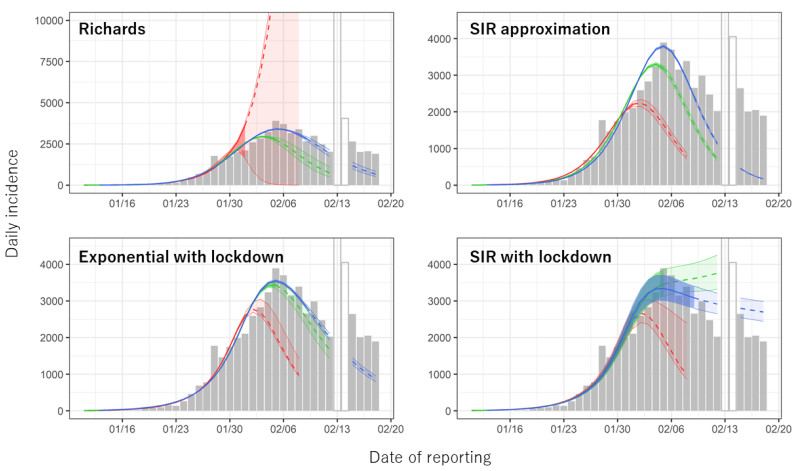
Forecasting future epidemics helps inform policy decisions regarding interventions. During the early coronavirus disease 2019 epidemic period in January–February 2020, limited information was available, and it was too challenging to build detailed mechanistic models reflecting population behavior. This study compared the performance of phenomenological and mechanistic models for forecasting epidemics. For the former, we employed the Richards model and the approximate solution of the susceptible–infected–recovered (SIR) model. For the latter, we examined the exponential growth (with lockdown) model and SIR model with lockdown. The phenomenological models yielded higher root mean square error (RMSE) values than the mechanistic models. When using the numbers from reported data for February 1 and 5, the Richards model had the highest RMSE, whereas when using the February 9 data, the SIR approximation model was the highest. The exponential model with a lockdown effect had the lowest RMSE, except when using the February 9 data. Once interventions or other factors that influence transmission patterns are identified, they should be additionally taken into account to improve forecasting.

References

[1]	WHO, Novel Coronavirus (2019-nCoV) Situation Report - 1, WHO, 2020. Available from: https://www.who.int/docs/default-source/coronaviruse/situation-reports/20200121-sitrep-1-2019-ncov.pdf?sfvrsn=20a99c10_4.
[2]	WHO, Novel Coronavirus (2019-nCoV) Situation Report – 3, WHO, 2020. Available from: https://www.who.int/docs/default-source/coronaviruse/situation-reports/20200123-sitrep-3-2019-ncov.pdf?sfvrsn=d6d23643_8.
[3]	The Paper, Xiangyang Railway Station is closed, the last prefecture-level city in Hubei Province is "closed", Shanghai Oriental Press, 2020. Available from: https://www.thepaper.cn/newsDetail_forward_5671283.
[4]	D. B. Taylor, A timeline of the coronavirus pandemic, New York Times, 2020. Available from: https://www.nytimes.com/article/coronavirus-timeline.html.
[5]	WHO-PRC Joint Misson, Report of the WHO-China joint mission on coronavirus disease 2019 (COVID-19), WHO, 2020. Available from: https://www.who.int/docs/default-source/coronaviruse/who-china-joint-mission-on-covid-19-final-report.pdf.
[6]	BBC, Coronavirus: people of Wuhan allowed to leave after lockdown, BBC, 2020. Available from: https://www.bbc.com/news/world-asia-china-52207776.
[7]	WHO, WHO Coronavirus Disease (COVID-19) Dashboard, WHO, 2021. Available from: https://covid19.who.int/region/wpro/country/cn.
[8]	C. S. Lutz, M. P. Huynh, M. Schroeder, S. Anyatonwu, F. S. Dahlgren, G. Danyluk, et al., Applying infectious disease forecasting to public health: A path forward using influenza forecasting examples, BMC Public Health, 19 (2019), 1659. doi: 10.1186/s12889-019-7966-8. doi: 10.1186/s12889-019-7966-8
[9]	L. S. Fischer, S. Santibanez, R. J. Hatchett, D. B. Jernigan, L. A. Meyers, P. G. Thorpe, et al., CDC grand rounds: Modeling and public health decision-making, Morb. Mortal. Wkly. Rep., 65 (2016), 1374–1377. doi: 10.15585/mmwr.mm6548a4. doi: 10.15585/mmwr.mm6548a4
[10]	K. Hayashi, T. Kayano, S. Sorano, H. Nishiura, Hospital caseload demand in the presence of interventions during the COVID-19 pandemic: a modeling study, J. Clin. Med., 9 (2020), 3065. doi: 10.3390/jcm9103065. doi: 10.3390/jcm9103065
[11]	J. T. Wu, K. Leung, G. M. Leung, Nowcasting and forecasting the potential domestic and international spread of the 2019-nCoV outbreak originating in Wuhan, China: A modelling study, Lancet, 395 (2020), 689–697. doi: 10.1016/S0140-6736(20)30260-9. doi: 10.1016/S0140-6736(20)30260-9
[12]	K. Roosa, Y. Lee, R. Luo, A. Kirpich, R. Rothenberg, M. James, et al., Short-term forecasts of the COVID-19 epidemic in Guangdong and Zhejiang, China: February 13–23, 2020. J. Clin. Med., 9 (2020), 596. doi: 10.3390/jcm9020596. doi: 10.3390/jcm9020596
[13]	K. Roosa, Y. Lee, R. Luo, A. Kirpich, R. Rothenberg, J. M. Hyman, et al., Real-time forecasts of the COVID-19 epidemic in China from February 5th to February 24th, 2020. Infect. Dis. Model., 5 (2020), 256–263. doi: 10.1016/j.idm.2020.02.002. doi: 10.1016/j.idm.2020.02.002
[14]	G. Chowell, D. Hincapie-Palacio, J. Ospina, B. Pell, A. Tariq, S. Dahal, et al., Using phenomenological models to characterize transmissibility and forecast patterns and final burden of Zika epidemics, PLoS Curr., 8 (2016), ecurrents.outbreaks.f14b2217c902f453d9320a43a35b9583. doi: 10.1371/currents.outbreaks.f14b2217c902f453d9320a43a35b9583. doi: 10.1371/currents.outbreaks.f14b2217c902f453d9320a43a35b9583
[15]	B. Pell, Y. Kuang, C. Viboud, G. Chowell, Using phenomenological models for forecasting the 2015 Ebola challenge. Epidemics, 22 (2018), 62–70. doi: 10.1016/j.epidem.2016.11.002. doi: 10.1016/j.epidem.2016.11.002
[16]	N. Balak, D. Inan, M. Ganau, C. Zoia, S. Sönmez, B. Kurt, et al., A simple mathematical tool to forecast COVID-19 cumulative case numbers, Clin. Epidemiol. Glob. Health, 12 (2021), 100853. doi: 10.1016/j.cegh.2021.100853. doi: 10.1016/j.cegh.2021.100853
[17]	F. Y. Hsieh, D. A. Bloch, M. D. Larsen, A simple method of sample size calculation for linear and logistic regression, Stat. Med., 17 (1998), 1623–1634. doi: 10.1002/(sici)1097-0258(19980730)17:14<1623::aid-sim871>3.0.co; 2-s. doi: 10.1002/(sici)1097-0258(19980730)17:14<1623::aid-sim871>3.0.co;2-s
[18]	Y.-H. Hsieh, Richards model: A simple procedure for real-time prediction of outbreak severity, in Modeling and Dynamics of Infectious Diseases (eds. Z. Ma, Y. Zhou and J. Wu), World Scientific Pub. Co. Inc., (2009), 216–236. doi: 10.1142/9789814261265_0009.
[19]	K. Roosa, A. Tariq, P. Yan, J. M. Hyman, G. Chowell, Multi-model forecasts of the ongoing Ebola epidemic in the Democratic Republic of Congo, March-October 2019, J. R. Soc. Interface, 17 (2020), 20200447. doi: 10.1098/rsif.2020.0447. doi: 10.1098/rsif.2020.0447
[20]	F. J. Richards, A flexible growth function for empirical use, J. Exp. Bot., 10 (1959), 290–301. doi: 10.1093/jxb/10.2.290. doi: 10.1093/jxb/10.2.290
[21]	M. J. Keeling, P. Rohani, Introduction to simple epidemic models, in Modeling Infectious Diseases in Humans and Animals, Princeton University Press, (2008), 15–53. doi: 10.2307/j.ctvcm4gk0.
[22]	N. T. Bailey, General epidemics, in The Mathematical Theory of Infectious Diseases, 2nd ed, Hafner Press, (1975), 81–102.
[23]	H. Nishiura, N. M. Linton, A.R. Akhmetzhanov, Serial interval of novel coronavirus (COVID-19) infections, Int. J. Infect. Dis., 93 (2020), 284–286. doi: 10.1016/j.ijid.2020.02.060. doi: 10.1016/j.ijid.2020.02.060
[24]	W. O. Kermack, A. G. Mckendrick, A contribution to the mathematical theory of epidemics, Proc. R. Soc. A, 115 (1927), 700–721. doi: 10.1098/rspa.1927.0118. doi: 10.1098/rspa.1927.0118
[25]	S. Jung, A. R. Akhmetzhanov, K. Hayashi, N. M. Linton, Y. Yang, B. Yuan, et al., Real-time estimation of the risk of death from novel coronavirus (COVID-19) infection: Inference using exported cases, J. Clin. Med., 9 (2020), 523. doi: 10.3390/jcm9020523. doi: 10.3390/jcm9020523
[26]	J. Wallinga, M. Lipsitch, How generation intervals shape the relationship between growth rates and reproductive numbers. Proc. R. Soc. B, 274 (2007), 599–604. doi: 10.1098/rspb.2006.3754. doi: 10.1098/rspb.2006.3754
[27]	H. Nishiura, T. Kobayashi, Y. Yang, K. Hayashi, T. Miyama, R. Kinoshita, et al., The rate of underascertainment of novel coronavirus (2019-nCoV) infection: Estimation using Japanese passengers data on evacuation flights, J. Clin. Med., 9 (2020), 419. doi: 10.3390/jcm9020419. doi: 10.3390/jcm9020419
[28]	N. M. Linton, T. Kobayashi, Y. Yang, K. Hayashi, A. R. Akhmetzhanov, S. Jung, et al., Incubation period and other epidemiological characteristics of 2019 novel coronavirus infections with right truncation: A statistical analysis of publicly available case data, J. Clin. Med., 9 (2020), 538. doi: 10.3390/jcm9020538. doi: 10.3390/jcm9020538
[29]	K. Leung, J. T. Wu, D. Liu, G. M. Leung, First-wave COVID-19 transmissibility and severity in China outside Hubei after control measures, and second-wave scenario planning: A modelling impact assessment. Lancet, 395 (2020), 1382–1393. doi: 10.1016/S0140-6736(20)30746-7. doi: 10.1016/S0140-6736(20)30746-7
[30]	G. Chowell, Fitting dynamic models to epidemic outbreaks with quantified uncertainty: A primer for parameter uncertainty, identifiability, and forecasts, Infect. Dis. Model., 2 (2017), 379–398. doi: 10.1016/j.idm.2017.08.001. doi: 10.1016/j.idm.2017.08.001
[31]	31. R Core Team, R: A language and environment for statistical computing, R Foundation for Statistical Computing, 2020. Available from: https://www.R-project.org/.
[32]	M. Li, J. Dushoff, B. M. Bolker, Fitting mechanistic epidemic models to data: A comparison of simple Markov chain Monte Carlo approaches, Stat. Methods Med. Res., 27 (2018), 1956–1967. doi: 10.1177/0962280217747054. doi: 10.1177/0962280217747054
[33]	D. W. Shanafelt, G. Jones, M. Lima, C. Perrings, G. Chowell, Forecasting the 2001 Foot-and-Mouth Disease epidemic in the UK, Ecohealth, 15 (2018), 338–347. doi: 10.1007/s10393-017-1293-2. doi: 10.1007/s10393-017-1293-2
[34]	W. Liu, S. Tang, Y. Xiao, Model selection and evaluation based on emerging infectious disease data sets including A/H1N1 and Ebola, Comput. Math. Methods Med., 2015 (2015), 207105. doi: 10.1155/2015/207105. doi: 10.1155/2015/207105
[35]	Y. H. Hsieh, Temporal course of 2014 Ebola virus disease (EVD) outbreak in West Africa elucidated through morbidity and mortality data: A tale of three countries, PLoS One, 10 (2015) 1–12. doi: 10.1371/journal.pone.0140810. doi: 10.1371/journal.pone.0140810
[36]	A. V. Tkachenko, S. Maslov, A. Elbanna, G. N. Wong, Z. J. Weiner, N. Goldenfeld, Time-dependent heterogeneity leads to transient suppression of the COVID-19 epidemic, not herd immunity, Proc. Natl. Acad. Sci. USA, 118 (2021), e2015972118. doi: 10.1073/PNAS.2015972118. doi: 10.1073/PNAS.2015972118
[37]	COVIDSurg Collaborative, GlobalSurg Collaborative, SARS-CoV-2 vaccination modelling for safe surgery to save lives: data from an international prospective cohort study, Br. J. Surg., 108 (2021), 1056–1063. doi: 10.1093/bjs/znab101.
[38]	B. F. Maier, D. Brockmann, Effective containment explains subexponential growth in recent confirmed COVID-19 cases in China, Science, 368 (2020), 742–746. doi: 10.1126/science.abb4557. doi: 10.1126/science.abb4557
[39]	M. Djordjevic, M. Djordjevic, B. Ilic, S. Stojku, I. Salom, Understanding infection progression under strong control measures through universal COVID-19 growth signatures, Glob. Chall., 5 (2021), 2000101. doi: 10.1002/gch2.202000101. doi: 10.1002/gch2.202000101

mbe-19-02-096 Supplementary.docx

Reader Comments

your name:*

Email:*
© 2022 the Author(s), licensee AIMS Press. This is an open access article distributed under the terms of the Creative Commons Attribution License (http://creativecommons.org/licenses/by/4.0)