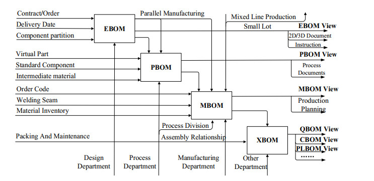
The bill of materials (BOM) runs through all stages of the life cycle of manufacturing products, which is the core of manufacturing enterprises. With increasing complexity of modern manufacturing engineering and widespread using of intelligent manufacturing technology, the BOM data keeps rising and transformation process is increasingly frequent and complicated. In order to improve efficiency of BOM management and ensure the diversity, accuracy and consistency of BOM in the product development, the BOM multi-view integrated management and mapping method for complex products were researched. First, a complex product BOM integrated management framework and the evolution model based on multiple views were established which described the BOM integrated management mechanism and transformation relationship among different BOMs. Subsequently, process of BOM transformation was analyzed, and a BOM transformation model was proposed. Moreover, a rule-based BOM multi-view mapping algorithm was proposed. With the rule definition and mathematical modelling for key components, the complex mapping principle was elaborated. Finally, the BOM multi-view transformation cases and the prototype system were illustrated and discussed, which verified the feasibility and versatility of model and method.
Citation: Jun Chen, Yuan Xiao, Gangfeng Wang, Biao Guo. Research on the integrated management and mapping method of BOM multi-view for complex products[J]. Mathematical Biosciences and Engineering, 2023, 20(7): 12682-12699. doi: 10.3934/mbe.2023565
The bill of materials (BOM) runs through all stages of the life cycle of manufacturing products, which is the core of manufacturing enterprises. With increasing complexity of modern manufacturing engineering and widespread using of intelligent manufacturing technology, the BOM data keeps rising and transformation process is increasingly frequent and complicated. In order to improve efficiency of BOM management and ensure the diversity, accuracy and consistency of BOM in the product development, the BOM multi-view integrated management and mapping method for complex products were researched. First, a complex product BOM integrated management framework and the evolution model based on multiple views were established which described the BOM integrated management mechanism and transformation relationship among different BOMs. Subsequently, process of BOM transformation was analyzed, and a BOM transformation model was proposed. Moreover, a rule-based BOM multi-view mapping algorithm was proposed. With the rule definition and mathematical modelling for key components, the complex mapping principle was elaborated. Finally, the BOM multi-view transformation cases and the prototype system were illustrated and discussed, which verified the feasibility and versatility of model and method.

| [1] | P. Burcher, Bill of Materials, Wiley Encyclopedia of Management, John Wiley & Sons, Ltd, 2015. https://doi.org/10.1002/9781118785317.weom100187 |
| [2] |
S. Y. Jung, B. H. Kim, J. Oh, An integrated multi-BOM system for product data management, J. Korea Safety Manage. Sci., 17 (2012), 216–223. https://doi.org/10.7315/CADCAM.2012.216 doi: 10.7315/CADCAM.2012.216

|
| [3] |
G. Atharvan, S. Krishnamoorthy, A way forward towards a technology-driven development of industry 4.0 using big data analytics in 5G-enabled IIoT, Int. J. Commun. Syst., 35 (2022), 1–41. https://doi.org/10.1002/dac.5014 doi: 10.1002/dac.5014
|
| [4] |
A. O. Aydin, A. Güngör, Effective relational database approach to represent bills-of-materials, Int. J. Prod. Res., 43 (2005), 1143–1170. https://doi.org/10.1080/00207540512331336528 doi: 10.1080/00207540512331336528
|
| [5] |
X. Liu, X. Huang, Y. Ma, Q. Meng, Y. Meng, Research on xBOM for product whole life cycle, Comput. Integr. Manuf. Syst., 8 (2002), 983–987. https://doi.org/10.13196/j.cims.2002.12.60.liuxb.013 doi: 10.13196/j.cims.2002.12.60.liuxb.013
|
| [6] |
X. Huang, Y. Fan, Research on BOM views and BOM view mapping model, Chin. J. Mech. Eng., 41 (2005), 101–106. https://doi.org/10.3901/JME.2005.12.101 doi: 10.3901/JME.2005.12.101
|
| [7] |
F. Xiang, Y. Huang, Z. Zhang, G. Jiang, Y. Zuo, Research on ECBOM modeling and energy consumption evaluation based on BOM multi-view transformation, J. Ambient Intell. Hum. Comput., 10 (2019), 953–967. https://doi.org/10.1007/s12652-018-1053-3 doi: 10.1007/s12652-018-1053-3
|
| [8] |
C. Zhou, X. Liu, F. Xue, H. Bo, K. Li, Research on static service BOM transformation for complex products, Adv. Eng. Inf., 36 (2018), 146–162. https://doi.org/10.1016/j.aei.2018.02.008 doi: 10.1016/j.aei.2018.02.008
|
| [9] | T. Li, Research and implementation of version management method for product structure information tree, Appl. Res. Comput., 27 (2010), 3829–3833. |
| [10] | F. Liu, Optimization of multi-version distribution mode for directed acyclic graph structure, Comput. Eng., 37 (2011), 74–76. |
| [11] | S. M. Hou, Y. X. Liu, Version management model of collaborative design based on theory of polychromatic sets, J. Northeast. Univ. (Nat. Sci.), 31 (2010), 427–431. |
| [12] | H. Zhang, S. Y. Shi, PLM-oriented BOM data management and practice, Manuf. Autom., 40 (2018), 30–34. |
| [13] |
J. Chen, G. F. Wang, An improved polychromatic graphs-based BOM multi-view management and version control method for complex products, Math. Biosci. Eng., 18 (2021), 712–726. https://doi.org/10.3934/mbe.2021038 doi: 10.3934/mbe.2021038
|
| [14] | N. C. Xia, Managing and mapping method for BOM multiple-view based on transform-table, J. Shanghai Jiaotong Univ., 42 (2008), 584–589. |
| [15] |
S. Y. Cai, Research on BOM multi-view mapping method orient to aircraft in-service data management, J. Phys. Conf. Ser., 1550 (2020), 032124. https://doi.org/10.1088/1742-6596/1550/3/032124 doi: 10.1088/1742-6596/1550/3/032124
|
| [16] | H. Zhang, J. J. Wu, Research on assembly BOM conversion method for information integration, J. Jiangsu Univ. Sci. Technol, 34 (2020), 41–48. |
| [17] | Z. Q. Wei, X. K. Wang, BOM multi-view mapping of product based on a single data source, J. Tsinghua Univ. (Sci. Technol.), 42 (2002), 802–805. |
| [18] | J. J. Yan, Z. X. Yang, Research on structure mapping method of BOM multi-view, Modular Mach. Tool Autom. Manuf. Tech., 52 (2020), 27–30. |
| [19] |
M. Liu, J. Lai, W. Shen, A method for transformation of engineering bill of materials to maintenance bill of materials, Rob. Comput. Integr. Manuf., 30 (2014), 142–149. https://doi.org/10.1016/j.rcim.2013.09.008 doi: 10.1016/j.rcim.2013.09.008
|
| [20] | Q. H. Liu, Method of BOM multi-view transformation based on configurable rule, Comput. Eng. Design, 33 (2012), 3418–3424. |
| [21] | H. Jiang, BOM-oriented manufacturing process system, Aeronaut. Manuf. Technol., 10 (2003), 33–35. |
| [22] | J. Y. Wang, Research on PBOM management system based on the PDM, Mach. Build. Autom., 45 (2016), 130–132. |
| [23] |
A. V. Singh, M. Varma, P. Laux, S. Choudhary, A. K. Datusalia, N. Gupta, et al., Artificial intelligence and machine learning disciplines with the potential to improve the nanotoxicology and nanomedicine fields: a comprehensive review, Arch. Toxicol., 97 (2023), 963–979. https://doi.org/10.1007/s00204-023-03471-x doi: 10.1007/s00204-023-03471-x
|
| [24] |
M. A. Abam, New constructions of SSPDs and their applications, Comput. Geom., 45 (2012), 200–214. https://doi.org/10.1016/j.comgeo.2011.12.003 doi: 10.1016/j.comgeo.2011.12.003
|
| [25] |
A. V. Singh, D. Rosenkranz, M. H. D. Ansari, R. Singh, A. Kanase, S. P. Singh, et al., Artificial intelligence and machine learning empower advanced biomedical material design to toxicity prediction, Adv. Intell. Syst., 2 (2020), 2000084. https://doi.org/10.1002/aisy.202000084 doi: 10.1002/aisy.202000084
|


Figures(10)

Jun Chen, Yuan Xiao, Gangfeng Wang, Biao Guo. Research on the integrated management and mapping method of BOM multi-view for complex products[J]. Mathematical Biosciences and Engineering, 2023, 20(7): 12682-12699. doi: 10.3934/mbe.2023565


 DownLoad: