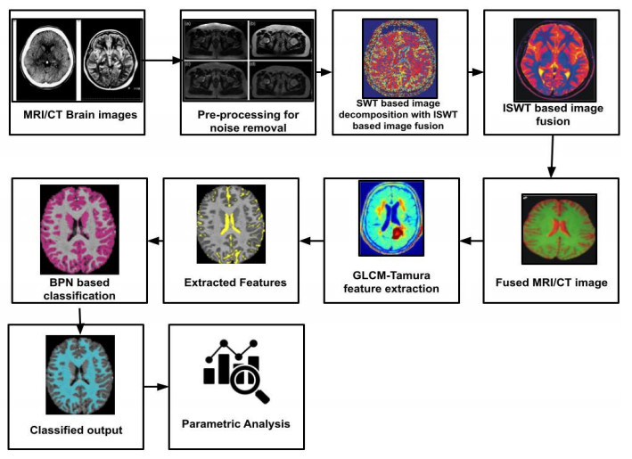
Most challenging task in medical image analysis is the detection of brain tumours, which can be accomplished by methodologies such as MRI, CT and PET. MRI and CT images are chosen and fused after preprocessing and SWT-based decomposition stage to increase efficiency. The fused image is obtained through ISWT. Further, its features are extracted through the GLCM-Tamura method and fed to the BPN classifier. Will employ supervised learning with a non-knowledge-based classifier for picture classification. The classifier utilized Trained databases of the tumour as benign or malignant from which the tumour region is segmented via k-means clustering. After the software needs to be implemented, the health status of the patients is notified through GSM. Our method integrates image fusion, feature extraction, and classification to distinguish and further segment the tumour-affected area and to acknowledge the affected person. The experimental analysis has been carried out regarding accuracy, precision, recall, F-1 score, RMSE and MAP.
Citation: R. Bhavani, K. Vasanth. Brain image fusion-based tumour detection using grey level co-occurrence matrix Tamura feature extraction with backpropagation network classification[J]. Mathematical Biosciences and Engineering, 2023, 20(5): 8727-8744. doi: 10.3934/mbe.2023383
Most challenging task in medical image analysis is the detection of brain tumours, which can be accomplished by methodologies such as MRI, CT and PET. MRI and CT images are chosen and fused after preprocessing and SWT-based decomposition stage to increase efficiency. The fused image is obtained through ISWT. Further, its features are extracted through the GLCM-Tamura method and fed to the BPN classifier. Will employ supervised learning with a non-knowledge-based classifier for picture classification. The classifier utilized Trained databases of the tumour as benign or malignant from which the tumour region is segmented via k-means clustering. After the software needs to be implemented, the health status of the patients is notified through GSM. Our method integrates image fusion, feature extraction, and classification to distinguish and further segment the tumour-affected area and to acknowledge the affected person. The experimental analysis has been carried out regarding accuracy, precision, recall, F-1 score, RMSE and MAP.

| [1] |
D. Sara, A. K. Mandava, A. Kumar, S. Duela, A. Jude, Hyperspectral and multispectral image fusion techniques for high-resolution applications: A review, Earth Sci. Inf., 14 (2021), 1685–1705. https://doi.org/10.1007/s12145-021-00621-6 doi: 10.1007/s12145-021-00621-6

|
| [2] |
X. Feng, L. He, Q. Cheng, X. Long, Y. Yuan, Hyperspectral and multispectral remote sensing image fusion based on endmember spatial information, Remote Sens., 12 (2020), 1009. https://doi.org/10.3390/rs12061009 doi: 10.3390/rs12061009
|
| [3] |
U. Subramaniam, M. M. Subashini, D. Almakhles, A. Karthick, S. Manoharan, An expert system for COVID-19 infection tracking in lungs using image processing and deep learning techniques, BioMed Res. Int., 2021 (2021), 1–17. https://doi.org/10.1155/2021/1896762 doi: 10.1155/2021/1896762
|
| [4] |
S. S. Ganesh, G. Kannayeram, A. Karthick, M. Muhibbullah, A novel context-aware joint segmentation and classification framework for glaucoma detection, Comput. Math. Methods Med., 2021 (2021), 1–19. https://doi.org/10.1155/2021/2921737 doi: 10.1155/2021/2921737
|
| [5] |
T. Saba, A. S. Mohamed, M. El-Affendi, J. Amin, M. Sharif, Brain tumour detection using fusion of handcrafted and deep learning features, Cognit. Syst. Res., 59 (2020), 221–230. https://doi.org/10.1016/j.cogsys.2019.09.007 doi: 10.1016/j.cogsys.2019.09.007
|
| [6] |
X. Liu, A. Yu, X. Wei, Z. Pan, J. Tang, Multimodal MR image synthesis using gradient prior and adversarial learning, IEEE J. Sel. Top. Signal Process., 14 (2020), 1176–1188. https://doi.org/10.1109/JSTSP.2020.3013418 doi: 10.1109/JSTSP.2020.3013418
|
| [7] |
M. Sharif, J. Amin, M. Raza, M. Yasmin, S. C. Satapathy, An integrated design of particle swarm optimization (PSO) with the fusion of features for detection of brain tumor, Pattern Recognit. Lett., 129 (2020), 150–157. https://doi.org/10.1016/j.patrec.2019.11.017 doi: 10.1016/j.patrec.2019.11.017
|
| [8] |
X. Liu, Z. Guo, J. Cao, J. Tang, MDC-net: A new convolutional neural network for nucleus segmentation in histopathology images with distance maps and contour information, Comput. Biol. Med., 135 (2021), 104543. https://doi.org/10.1016/j.compbiomed.2021.104543 doi: 10.1016/j.compbiomed.2021.104543
|
| [9] |
Z. Hu, J. Tang, Z. Wang, K. Zhang, L. Zhang, Q. Sun, Deep learning for image-based cancer detection and Diagnosis—A survey, Pattern Recognit., 83 (2018), 134–149. https://doi.org/10.1016/j.patcog.2018.05.014 doi: 10.1016/j.patcog.2018.05.014
|
| [10] |
H. Kaur, D. Koundal, V. Kadyan, N. Kaur, K. Polat, Automated Multimodal image fusion for brain tumor detection, J. Artif. Intell. Syst., 3 (2021), 68–82. https://doi.org/10.33969/AIS.2021.31005 doi: 10.33969/AIS.2021.31005
|
| [11] |
J. Amin, M. Sharif, N. Gul, M. Yasmin, S. A. Shad, Brain tumor classification based on DWT fusion of MRI sequences using convolutional neural network, Pattern Recognit. Lett., 129 (2020), 115–122. https://doi.org/10.1016/j.patrec.2019.11.016 doi: 10.1016/j.patrec.2019.11.016
|
| [12] |
R. Nanmaran, S. Srimathi, G. Yamuna, S. Thanigaivel, A. S. Vickram, A. K. Priya, et al., Investigating the role of image fusion in brain tumor classification models based on machine learning algorithm for personalized medicine, Comput. Math. Methods Med., 2022 (2022), 1–13. https://doi.org/10.1155/2022/7137524 doi: 10.1155/2022/7137524
|
| [13] |
A. Selvapandian, K. Manivannan, Fusion based Glioma brain tumor detection and segmentation using ANFIS classification, Comput. Methods Programs Biomed., 166 (2018), 33–38. https://doi.org/10.1016/j.cmpb.2018.09.006 doi: 10.1016/j.cmpb.2018.09.006
|
| [14] |
S. Preethi, P. Aishwarya, An efficient wavelet-based image fusion for brain tumor detection and segmentation over PET and MRI image, Multimed Tools Appl., 80 (2021), 14789–14806. https://doi.org/10.1007/s11042-021-10538-3 doi: 10.1007/s11042-021-10538-3
|
| [15] |
P. M. Kumar, R. Saravanakumar, A. Karthick, V. Mohanavel, Artificial neural network-based output power prediction of grid-connected semitransparent photovoltaic system, Environ. Sci. Pollut. Res., 29 (2022), 10173–10182. https://doi.org/10.1007/s11356-021-16398-6 doi: 10.1007/s11356-021-16398-6
|
| [16] |
N. Jeevanand, P. A. Verma, S. Saran, Fusion of hyperspectral and multispectral imagery with regression Kriging and the Lulu operators: A comparison, Int. Arch. Photogramm. Remote Sens. Spatial Inf. Sci., 5 (2018), 583–588. https://doi.org/10.5194/isprs-archives-XLⅡ-5-583-2018 doi: 10.5194/isprs-archives-XLⅡ-5-583-2018
|
| [17] |
V. Chandran, M. G. Sumithra, A. Karthick, T. George, M. Deivakani, B. Elakkiya, et al., Diagnosis of cervical cancer based on ensemble deep learning network using colposcopy images, BioMed Res. Int., 2021 (2021), 1–15. https://doi.org/10.1155/2021/5584004 doi: 10.1155/2021/5584004
|
| [18] | D. Jiang, D. Zhuang, Y. Huang, J. Fu, Survey of multispectral image fusion techniques in remote sensing applications, in Image Fusion and its Applications (ed. Y. Zheng), IntechOpen, (2011), 1–23. |
| [19] |
R. Kabilan, V. Chandran, J. Yogapriya, A. Karthick, P. P. Gandhi, V. Mohanavel, et al., Short-term power prediction of building integrated photovoltaic (BIPV) system based on machine learning algorithms, Int. J. Photoenergy, 2021 (2021), 1–11. https://doi.org/10.1155/2021/5582418 doi: 10.1155/2021/5582418
|
| [20] | B. K. Umri, M. W. Akhyari, K. Kusrini, Detection of covid-19 in chest X-ray image using CLAHE and convolutional neural network, in 2020 2nd International Conference on Cybernetics and Intelligent System (ICORIS), IEEE, Manado, Indonesia, (2020), 1–5. https://doi.org/10.1109/ICORIS50180.2020.9320806 |
| [21] |
V. Chandran, C. K. Patil, A. M. Manoharan, A. Ghosh, M. G. Sumithra, A. Karthick, et al., Wind power forecasting based on time series model using deep machine learning algorithms, Mater. Today Proc., 47 (2021), 115–126. https://doi.org/10.1016/j.matpr.2021.03.728 doi: 10.1016/j.matpr.2021.03.728
|
| [22] |
V. Chandran, C. K. Patil, A. Karthick, D. Ganeshaperumal, R. Rahim, A. Ghosh, State of charge estimation of lithium-ion battery for electric vehicles using machine learning algorithms, WEVJ, 12 (2021), 38. https://doi.org/10.3390/wevj12010038 doi: 10.3390/wevj12010038
|


Figures(6) / Tables(2)

R. Bhavani, K. Vasanth. Brain image fusion-based tumour detection using grey level co-occurrence matrix Tamura feature extraction with backpropagation network classification[J]. Mathematical Biosciences and Engineering, 2023, 20(5): 8727-8744. doi: 10.3934/mbe.2023383


 DownLoad: