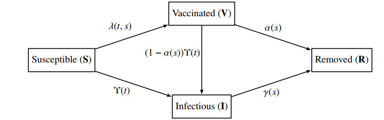
The Dynamical Survival Analysis (DSA) is a framework for modeling epidemics based on mean field dynamics applied to individual (agent) level history of infection and recovery. Recently, the Dynamical Survival Analysis (DSA) method has been shown to be an effective tool in analyzing complex non-Markovian epidemic processes that are otherwise difficult to handle using standard methods. One of the advantages of Dynamical Survival Analysis (DSA) is its representation of typical epidemic data in a simple although not explicit form that involves solutions of certain differential equations. In this work we describe how a complex non-Markovian Dynamical Survival Analysis (DSA) model may be applied to a specific data set with the help of appropriate numerical and statistical schemes. The ideas are illustrated with a data example of the COVID-19 epidemic in Ohio.
Citation: Colin Klaus, Matthew Wascher, Wasiur R. KhudaBukhsh, Grzegorz A. Rempała. Likelihood-Free Dynamical Survival Analysis applied to the COVID-19 epidemic in Ohio[J]. Mathematical Biosciences and Engineering, 2023, 20(2): 4103-4127. doi: 10.3934/mbe.2023192
The Dynamical Survival Analysis (DSA) is a framework for modeling epidemics based on mean field dynamics applied to individual (agent) level history of infection and recovery. Recently, the Dynamical Survival Analysis (DSA) method has been shown to be an effective tool in analyzing complex non-Markovian epidemic processes that are otherwise difficult to handle using standard methods. One of the advantages of Dynamical Survival Analysis (DSA) is its representation of typical epidemic data in a simple although not explicit form that involves solutions of certain differential equations. In this work we describe how a complex non-Markovian Dynamical Survival Analysis (DSA) model may be applied to a specific data set with the help of appropriate numerical and statistical schemes. The ideas are illustrated with a data example of the COVID-19 epidemic in Ohio.

| [1] |
L. An, V. R. Grimm, A. Sullivan, B. L. Turner II, N. Malleson, A. Heppenstall, et al., Challenges, tasks, and opportunities in modeling agent-based complex systems, Ecolog. Model., 457 (2021), 109685. https://doi.org/10.1016/j.ecolmodel.2021.109685 doi: 10.1016/j.ecolmodel.2021.109685

|
| [2] | W. R. KhudaBukhsh, B. S. Choi, E. Kenah, G. A. Rempała, Survival dynamical systems: Individual-level survival analysis from population-level epidemic models, Interface Focus, 10 (2020). https://doi.org/10.1098/rsfs.2019.0048 |
| [3] | F. Di Lauro, W. R. KhudaBukhsh, I. Z. Kiss, E. Kenah, M. Jensen, G. A. Rempała, Dynamic survival analysis for non-markovian epidemic models. J. Royal Soc. Interf., 19 (2022), 20220124. https://doi.org/10.1098/rsif.2022.0124 |
| [4] | B. S. Choi, S. Busch, D. Kazadi, B. Ilunga, E. Okitolonda, Y. Dai, et al., Modeling outbreak data: Analysis of a 2012 Ebola virus disease epidemic in DRC, Biomath, 8 (2019). https://doi.org/10.11145/j.biomath.2019.10.037 |
| [5] | H. Vossler, P. Akilimali, Y. H. Pan, W. R. KhudaBukhsh, E. Kenah, G. A. Rempała, Analysis of individual-level epidemic data: Study of 2018-2020 Ebola outbreak in Democratic Republic of the Congo, Sci. Rep., 12 (2022). https://doi.org/10.1038/s41598-022-09564-4 |
| [6] | W. R. KhudaBukhsh, S. K. Khalsa, E. Kenah, G. A. Rempala, J. H. Tien, COVID-19 dynamics in an Ohio prison,, medRxiv, 2021. Available from: https://www.medrxiv.org/content/early/2021/01/15/2021.01.14.21249782 |
| [7] | M. Wascher, P. M. Schnell, W. R. KhudaBukhsh, M. Quam, J. H. Tien, G. A. Rempała, Monitoring sars-cov-2 transmission and prevalence in populations under repeated testing, 2021. Available from: https://www.medrxiv.org/content/10.1101/2021.06.22.21259342v1 |
| [8] | I. Somekh, W. R. KhudaBukhsh, E. D. Root, G. A. Rempała, E. Sim{ o}es, E. Somekh, Quantifying the population-level effect of the COVID-19 mass vaccination campaign in Israel: A modeling study, Open Forum Infect. Diseases, 9 (2022). https://doi.org/10.1093/ofid/ofac087 |
| [9] |
E. Kenah, Contact intervals, survival analysis of epidemic data, and estimation of $R_0$, Biostatistics, 12 (2011), 548–566. https://doi.org/10.1093/biostatistics/kxq068 doi: 10.1093/biostatistics/kxq068
|
| [10] | N. G. van Kampen, Remarks on Non-Markov Processes, Brazilian J. Phys., 28 (1998). |
| [11] | R. Ferrière, V. C. Tran, Stochastic and deterministic models for age-structured populations with genetically variable traits, In CANUM 2008, volume 27 of ESAIM Proc., pages 289–310. EDP Sci., Les Ulis, 2009. https://doi.org/10.1051/proc/2009033 |
| [12] |
E. Franco, M. Gyllenberg, O. Diekmann, One dimensional reduction of a renewal equation for a measure-valued function of time describing population dynamics, Acta Appl. Math., 175 (2021), 12. https://doi.org/10.1007/s10440-021-00440-3 doi: 10.1007/s10440-021-00440-3
|
| [13] |
J. M. Hyman, J. Li, Infection-age structured epidemic models with behavior change or treatment, J. Biol. Dynam., 1 (2007), 109–131. https://doi.org/10.1080/17513750601040383 doi: 10.1080/17513750601040383
|
| [14] |
N. Sherborne, J. C. Miller, K. B. Blyuss, I. Z. Kiss, Mean-field models for non-markovian epidemics on networks, J. Math. Biol., 76 (2018), 755–778. https://doi.org/10.1007/s00285-017-1155-0 doi: 10.1007/s00285-017-1155-0
|
| [15] |
V. C. Tran, Large population limit and time behaviour of a stochastic particle model describing an age-structured population, ESAIM. Probab. Stat., 12 (2008), 345–386. https://doi.org/10.1051/ps:2007052 doi: 10.1051/ps:2007052
|
| [16] | N. Fournier, S. Méléard, A microscopic probabilistic description of a locally regulated population and macroscopic approximations, Ann. Appl. Probab., 14 (2004), 1880–1919. |
| [17] |
W. R. KhudaBukhsh, H.-W. Kang, E. Kenah, G. Rempała, Incorporating age and delay into models for biophysical systems, Phys. Biol., 18 (2021), 10. https://doi.org/10.1088/1478-3975/abc2ab doi: 10.1088/1478-3975/abc2ab
|
| [18] | W. R. KhudaBukhsh, C. D Bastian, M. Wascher, C. Klaus, S. Y. Sahai, M. H. Weir, et al., Projecting covid-19 cases and subsequent hospital burden in ohio, medRxiv, 2022. Available from: https://www.medrxiv.org/content/10.1101/2022.07.27.22278117v1.full.pdf+html |
| [19] |
C. D. Bastian, G. A. Rempala, Throwing stones and collecting bones: Looking for poisson-like random measures, Math. Methods Appl. Sci., 43 (2020), 4658–4668. https://doi.org/10.1002/mma.6224 doi: 10.1002/mma.6224
|
| [20] | G. F. Webb, Theory of nonlinear age-dependent population dynamics, volume 89 of Monographs and Textbooks in Pure and Applied Mathematics. Marcel Dekker, Inc., New York, 1985. https://doi.org/10.1007/BF00250793 |
| [21] | M. Iannelli, M. Martcheva, F. A. Milner, Gender-structured population modeling, volume 31 of Frontiers in Applied Mathematics, Society for Industrial and Applied Mathematics (SIAM), Philadelphia, PA, 2005. |
| [22] | L. C. Evans, Partial differential equations, volume 19 of Graduate Studies in Mathematics, American Mathematical Society, Providence, RI, second edition, 2010. |
| [23] | E. DiBenedetto, Partial differential equations, Cornerstones. Birkhäuser Boston, Ltd., Boston, MA, second edition, 2010. |
| [24] | C Klaus, PDE-DSA github repository, 2022. Available from: https://github.com/klauscj68/PDE-Vax |
| [25] | J. Bezanson, A. Edelman, S. Karpinski, V. B. Shah, Julia: A fresh approach to numerical computing, SIAM Rev., 59 (2017), 65–98. |
| [26] | Ohio Department of Health, Ohio Department of Health COVID Dashboard, Available from: https://coronavirus.ohio.gov/wps/portal/gov/covid-19/dashboards/overview |
| [27] | Centers for Disease Control and Prevention (CDC), US Centers for Disease Control and Prevention: COVID-19 vaccinations in the United States, County, Available from: https://data.cdc.gov/Vaccinations/COVID-19-Vaccinations-in-the-United-States-County/8xkx-amqh |
| [28] | U. S. Census, County Population Totals 2010-2019, Available from: https://www.census.gov/data/datasets/time-series/demo/popest/2010s-counties-total.html |
| [29] | L. L. Schumaker, Spline functions: Computational Methods, Society for Industrial and Applied Mathematics, Philadelphia, PA, 2015. https://doi.org/10.1137/1.9781611973907 |
| [30] |
T. Kypraios, P. Neal, D. Prangle, A tutorial introduction to bayesian inference for stochastic epidemic models using approximate bayesian computation, {Math. Biosci.}, 287 (2017), 42–53. https://doi.org/10.1016/j.mbs.2016.07.001 doi: 10.1016/j.mbs.2016.07.001
|
| [31] | S..A. Sisson, Y. N. Fan, M. A. Beaumont, Handbook of Approximate Bayesian Computation, CRC Press, Boca Raton, FL, 2020. |
| [32] | Centers for Disease Control and Prevention (CDC), US Centers for Disease Control and Prevention: SARS-CoV-2 Variant Classifications and Definitions, Available from: https://www.cdc.gov/coronavirus/2019-ncov/variants/variant-classifications.html |
| [33] |
K. Koelle, M. A. Martin, R. Antia, B. Lopman, N. E. Dean, The changing epidemiology of sars-cov-2, Science, 375 (2022), 1116–1121. https://doi.org/10.1126/science.abm4915 doi: 10.1126/science.abm4915
|
| [34] |
M. O'Driscoll, G. R. Dos Santos, L. Wang, D. A. T. Cummings, A. S. Azman, J. Paireau, et al., Age-specific mortality and immunity patterns of SARS-CoV-2, Nature, 590 (2021), 140–145. https://doi.org/10.1038/s41586-020-2918-0 doi: 10.1038/s41586-020-2918-0
|
| [35] | I. Holmdahl, C. Buckee, Wrong but useful—what covid-19 epidemiologic models can and cannot tell us, New England J. Med., 383 (2020), 303–305. |
| [36] |
N. P. Jewell, J. A. Lewnard, B. L. Jewell, Predictive mathematical models of the COVID-19 Pandemic: Underlying principles and value of projections, JAMA, 323 (2020), 1893–1894. https://doi.org/10.1001/jama.2020.6585 doi: 10.1001/jama.2020.6585
|
| [37] |
N. Barda, D. Riesel, A. Akriv, J. Levy, U. Finkel, G. Yona, et al. Developing a COVID-19 mortality
risk prediction model when individual-level data are not available, Nat. Commun., 11 (2020), 4439. https://doi.org/10.1038/s41467-020-18297-9 doi: 10.1038/s41467-020-18297-9
|
| [38] |
C. Klaus, M. Wascher, W. R. KhudaBukhsh, J. H. Tien, G. A. Rempała, E. Kenah, Assortative mixing among vaccination groups and biased estimation of reproduction numbers, Lancet Infect. Diseases, 22 (2022), 579–581. https://doi.org/10.1016/S1473-3099(22)00155-4 doi: 10.1016/S1473-3099(22)00155-4
|
| [39] | O. A. Ladyženskaja, V. A. Solonnikov, N. N. Ural'ceva, Linear and quasilinear equations of parabolic type, in Translations of Mathematical Monographs, Vol. 23. American Mathematical Society, Providence, R.I., 1968. Translated from the Russian by S. Smith. |

Figures(7) / Tables(1)

Colin Klaus, Matthew Wascher, Wasiur R. KhudaBukhsh, Grzegorz A. Rempała. Likelihood-Free Dynamical Survival Analysis applied to the COVID-19 epidemic in Ohio[J]. Mathematical Biosciences and Engineering, 2023, 20(2): 4103-4127. doi: 10.3934/mbe.2023192


 DownLoad: