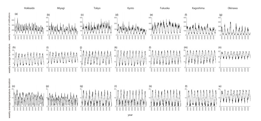
In Japan, major and minor bimodal seasonal patterns of varicella have been observed. To investigate the underlying mechanisms of seasonality, we evaluated the effects of the school term and temperature on the incidence of varicella in Japan. We analyzed epidemiological, demographic and climate datasets of seven prefectures in Japan. We fitted a generalized linear model to the number of varicella notifications from 2000 to 2009 and quantified the transmission rates as well as the force of infection, by prefecture. To evaluate the effect of annual variation in temperature on the rate of transmission, we assumed a threshold temperature value. In northern Japan, which has large annual temperature variations, a bimodal pattern in the epidemic curve was observed, reflecting the large deviation in average weekly temperature from the threshold value. This bimodal pattern was diminished with southward prefectures, gradually shifting to a unimodal pattern in the epidemic curve, with little temperature deviation from the threshold. The transmission rate and force of infection, considering the school term and temperature deviation from the threshold, exhibited similar seasonal patterns, with a bimodal pattern in the north and a unimodal pattern in the south. Our findings suggest the existence of preferable temperatures for varicella transmission and an interactive effect of the school term and temperature. Investigating the potential impact of temperature elevation that could reshape the epidemic pattern of varicella to become unimodal, even in the northern part of Japan, is required.
Citation: Ayako Suzuki, Hiroshi Nishiura. Seasonal transmission dynamics of varicella in Japan: The role of temperature and school holidays[J]. Mathematical Biosciences and Engineering, 2023, 20(2): 4069-4081. doi: 10.3934/mbe.2023190
In Japan, major and minor bimodal seasonal patterns of varicella have been observed. To investigate the underlying mechanisms of seasonality, we evaluated the effects of the school term and temperature on the incidence of varicella in Japan. We analyzed epidemiological, demographic and climate datasets of seven prefectures in Japan. We fitted a generalized linear model to the number of varicella notifications from 2000 to 2009 and quantified the transmission rates as well as the force of infection, by prefecture. To evaluate the effect of annual variation in temperature on the rate of transmission, we assumed a threshold temperature value. In northern Japan, which has large annual temperature variations, a bimodal pattern in the epidemic curve was observed, reflecting the large deviation in average weekly temperature from the threshold value. This bimodal pattern was diminished with southward prefectures, gradually shifting to a unimodal pattern in the epidemic curve, with little temperature deviation from the threshold. The transmission rate and force of infection, considering the school term and temperature deviation from the threshold, exhibited similar seasonal patterns, with a bimodal pattern in the north and a unimodal pattern in the south. Our findings suggest the existence of preferable temperatures for varicella transmission and an interactive effect of the school term and temperature. Investigating the potential impact of temperature elevation that could reshape the epidemic pattern of varicella to become unimodal, even in the northern part of Japan, is required.

| [1] |
A. M. Arvin, Varicella-zoster virus, Clin. Microbiol. Rev., 9 (1996), 361–381. https://doi.org/10.1128/CMR.9.3.361 doi: 10.1128/CMR.9.3.361

|
| [2] |
A. A. Gershon, J. Breuer, J. I. Cohen, R. J. Cohrs, M. D. Gershon, D. Gilden, et al., Varicella zoster virus infection, Nat. Rev. Dis. Primers, 1 (2015), 15016. https://doi.org/10.1038/nrdp.2015.16 doi: 10.1038/nrdp.2015.16
|
| [3] |
M. Marin, M. Marti, A. Kambhampati, S. M. Jeram, J. F. Seward, Global varicella vaccine effectiveness: A meta-analysis, Pediatrics, 137 (2016), e20153741. https://doi.org/10.1542/peds.2015-3741 doi: 10.1542/peds.2015-3741
|
| [4] |
A. Suzuki, H. Nishiura, Reconstructing the transmission dynamics of varicella in Japan: an elevation of age at infection, PeerJ, 10 (2022), e12767. https://doi.org/10.7717/peerj.12767 doi: 10.7717/peerj.12767
|
| [5] |
A. Suzuki, H. Nishiura, Transmission dynamics of varicella before, during and after the COVID-19 pandemic in Japan: A modelling study, Math. Biosci. Eng., 19 (2022), 5998–6012. https://doi.org/10.3934/mbe.2022280 doi: 10.3934/mbe.2022280
|
| [6] |
H. F. Gidding, M. Brisson, C. R. Macintyre, M. A. Burgess, Modelling the impact of vaccination on the epidemiology of varicella zoster virus in Australia, Aust. N. Z. J. Public Health, 29 (2005), 544–551. https://doi.org/10.1111/j.1467-842x.2005.tb00248.x doi: 10.1111/j.1467-842x.2005.tb00248.x
|
| [7] |
M. Karhunen, T. Leino, H. Salo, I. Davidkin, T. Kilpi, K. Auranen, Modelling the impact of varicella vaccination on varicella and zoster, Epidemiol. Infect., 138 (2010), 469–481. https://doi.org/10.1017/S0950268809990768 doi: 10.1017/S0950268809990768
|
| [8] |
F. Lienert, O. Weiss, K. Schmitt, U. Heininger, P. Guggisberg, Acceptance of universal varicella vaccination among Swiss pediatricians and general practitioners who treat pediatric patients, BMC Infect. Dis., 21 (2021), 12. https://doi.org/10.1186/s12879-020-05586-3 doi: 10.1186/s12879-020-05586-3
|
| [9] |
W. P. London, J. A. Yorke, Recurrent outbreaks of measles, chickenpox and mumps. I. Seasonal variation in contact rates, Am. J. Epidemiol., 98 (1973), 453–468. https://doi.org/10.1093/oxfordjournals.aje.a121575 doi: 10.1093/oxfordjournals.aje.a121575
|
| [10] |
N. C. Grassly, C. Fraser, Seasonal infectious disease epidemiology, Proc. Biol. Sci., 273 (2006), 2541–2550. https://doi.org/10.1098/rspb.2006.3604 doi: 10.1098/rspb.2006.3604
|
| [11] |
P. E. Fine, J. A. Clarkson, Measles in England and Wales--Ⅰ: An analysis of factors underlying seasonal patterns, Int. J. Epidemiol., 11 (1982), 5–14. https://doi.org/10.1093/ije/11.1.5 doi: 10.1093/ije/11.1.5
|
| [12] |
B. Finkenstädt, B. Grenfell, 2000 Time series modelling of childhood diseases: A dynamical systems approach, Appl. Statist., 49 (2000), 187–205. https://doi.org/10.1111/1467-9876.00187 doi: 10.1111/1467-9876.00187
|
| [13] |
D. He, D. J. Earn, The cohort effect in childhood disease dynamics, J. R. Soc. Interface, 13 (2016), 20160156. https://doi.org/10.1098/rsif.2016.0156 doi: 10.1098/rsif.2016.0156
|
| [14] |
C. Jackson, P. Mangtani, P. Fine, E. Vynnycky, The effects of school holidays on transmission of varicella zoster virus, England and Wales, 1967-2008, PLoS One, 9 (2014), e99762. https://doi.org/10.1371/journal.pone.0099762 doi: 10.1371/journal.pone.0099762
|
| [15] | D. L. Heymann, American Public Health Association, in Control of Communicable Diseases Manual (20th edition), American Public Health Association Publications, Washington, 2015. |
| [16] |
R. E. Baker, A. S. Mahmud, C. J. E. Metcalf, Dynamic response of airborne infections to climate change: predictions for varicella, Clim. Change, 148 (2018), 547–560. https://doi.org/10.1007/s10584-018-2204-4 doi: 10.1007/s10584-018-2204-4
|
| [17] | Statistical Handbook of Japan, Chapter 1 Land and Climate, 2021. Available from: https://www.stat.go.jp/english/data/handbook/c0117.html. |
| [18] | Japan Meteorological Agency, General Information on Climate of Japan. Available from: https://www.data.jma.go.jp/gmd/cpd/longfcst/en/tourist.html. |
| [19] | Ministry of Health, Labour and Welfare, Available from: https://www.mhlw.go.jp/stf/seisakunitsuite/bunya/kenkou_iryou/kenkou/kekkaku-kansenshou/kekkaku-kansenshou11/01.html#list05 (in Japanese). |
| [20] | Japan Meteorological Agency. Available from: https://www.data.jma.go.jp/obd/stats/etrn/ (in Japanese). |
| [21] |
K. Harigane, A. Sumi, K. Mise, N. Kobayashi, The role of temperature in reported chickenpox cases from 2000 to 2011 in Japan, Epidemiol. Infect., 143 (2015), 2666–2678. https://doi.org/10.1017/S095026881400363X doi: 10.1017/S095026881400363X
|
| [22] | National Institute of Population and Social Security Research, Population Projections for Japan. Available from: http://www.ipss.go.jp/pp-zenkoku/e/zenkoku_e2017/pp29_summary.pdf. |
| [23] |
T. Ozaki, Long-term clinical studies of varicella vaccine at a regional hospital in Japan and proposal for a varicella vaccination program, Vaccine, 31 (2013), 6155–6160. https://doi.org/10.1016/j.vaccine.2013.10.060 doi: 10.1016/j.vaccine.2013.10.060
|
| [24] |
O. N. Bjørnstad, B. F. Finkenstädt, B. T. Grenfell, Dynamics of measles epidemics: estimating scaling of transmission rates using a time series SIR model, Ecol. Monogr., 72 (2002), 169–184. https://doi.org/10.2307/3100023 doi: 10.2307/3100023
|
| [25] |
J. Shaman, V. E. Pitzer, C. Viboud, B. T. Grenfell, M. Lipsitch, Absolute humidity and the seasonal onset of influenza in the continental United States, PLoS Biol., 8 (2010), e1000316. https://doi.org/10.1371/journal.pbio.1000316 doi: 10.1371/journal.pbio.1000316
|
| [26] |
J. D. Tamerius, J. Shaman, W. J. Alonso, K. Bloom-Feshbach, C. K. Uejio, A. Comrie, et al., Environmental predictors of seasonal influenza epidemics across temperate and tropical climates, PLoS Pathog., 9 (2013), e1003194. https://doi.org/10.1371/journal.ppat.1003194 doi: 10.1371/journal.ppat.1003194
|
| [27] |
J. B. Axelsen, R. Yaari, B. T. Grenfell, L. Stone, Multiannual forecasting of seasonal influenza dynamics reveals climatic and evolutionary drivers, Proc. Natl. Acad. Sci.U. S. A., 111 (2014), 9538–9542. https://doi.org/10.1073/pnas.1321656111 doi: 10.1073/pnas.1321656111
|
| [28] |
A. C. Lowen, J. Steel, Roles of humidity and temperature in shaping influenza seasonality, J. Virol., 88 (2014), 7692–7695. https://doi.org/10.1128/JVI.03544-13 doi: 10.1128/JVI.03544-13
|
| [29] |
D. E. te Beest, M. van Boven, M. Hooiveld, C. van den Dool, J. Wallinga, Driving factors of influenza transmission in the Netherlands, Am. J. Epidemiol., 178 (2013), 1469–1477. https://doi.org/10.1093/aje/kwt132 doi: 10.1093/aje/kwt132
|
| [30] |
H. Yuan, S. C. Kramer, E. H. Y. Lau, B. J. Cowling, W. Yang, Modeling influenza seasonality in the tropics and subtropics, PLoS Comput. Biol., 17 (2021), e1009050. https://doi.org/10.1371/journal.pcbi.1009050 doi: 10.1371/journal.pcbi.1009050
|
| [31] |
S. T. Ali, B. J. Cowling, J. Y. Wong, D. Chen, S. Shan, E. H. Y. Lau, et al., Influenza seasonality and its environmental driving factors in mainland China and Hong Kong, Sci. Total Environ., 818 (2022), 151724. https://doi.org/10.1016/j.scitotenv.2021.151724 doi: 10.1016/j.scitotenv.2021.151724
|
| [32] |
N. Toyama, K. Shiraki, Epidemiology of herpes zoster and its relationship to varicella in Japan: A 10-year survey of 48,388 herpes zoster cases in Miyazaki prefecture, J. Med. Virol., 12 (2009), 2053–2058. https://doi.org/10.1002/jmv.21599 doi: 10.1002/jmv.21599
|


Figures(6) / Tables(2)

Ayako Suzuki, Hiroshi Nishiura. Seasonal transmission dynamics of varicella in Japan: The role of temperature and school holidays[J]. Mathematical Biosciences and Engineering, 2023, 20(2): 4069-4081. doi: 10.3934/mbe.2023190


 DownLoad: