As an important task in bioinformatics, protein secondary structure prediction (PSSP) is not only beneficial to protein function research and tertiary structure prediction, but also to promote the design and development of new drugs. However, current PSSP methods cannot sufficiently extract effective features. In this study, we propose a novel deep learning model WGACSTCN, which combines Wasserstein generative adversarial network with gradient penalty (WGAN-GP), convolutional block attention module (CBAM) and temporal convolutional network (TCN) for 3-state and 8-state PSSP. In the proposed model, the mutual game of generator and discriminator in WGAN-GP module can effectively extract protein features, and our CBAM-TCN local extraction module can capture key deep local interactions in protein sequences segmented by sliding window technique, and the CBAM-TCN long-range extraction module can further capture the key deep long-range interactions in sequences. We evaluate the performance of the proposed model on seven benchmark datasets. Experimental results show that our model exhibits better prediction performance compared to the four state-of-the-art models. The proposed model has strong feature extraction ability, which can extract important information more comprehensively.
Citation: Lu Yuan, Yuming Ma, Yihui Liu. Protein secondary structure prediction based on Wasserstein generative adversarial networks and temporal convolutional networks with convolutional block attention modules[J]. Mathematical Biosciences and Engineering, 2023, 20(2): 2203-2218. doi: 10.3934/mbe.2023102
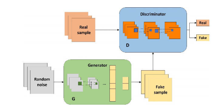
As an important task in bioinformatics, protein secondary structure prediction (PSSP) is not only beneficial to protein function research and tertiary structure prediction, but also to promote the design and development of new drugs. However, current PSSP methods cannot sufficiently extract effective features. In this study, we propose a novel deep learning model WGACSTCN, which combines Wasserstein generative adversarial network with gradient penalty (WGAN-GP), convolutional block attention module (CBAM) and temporal convolutional network (TCN) for 3-state and 8-state PSSP. In the proposed model, the mutual game of generator and discriminator in WGAN-GP module can effectively extract protein features, and our CBAM-TCN local extraction module can capture key deep local interactions in protein sequences segmented by sliding window technique, and the CBAM-TCN long-range extraction module can further capture the key deep long-range interactions in sequences. We evaluate the performance of the proposed model on seven benchmark datasets. Experimental results show that our model exhibits better prediction performance compared to the four state-of-the-art models. The proposed model has strong feature extraction ability, which can extract important information more comprehensively.

| [1] |
Y. Yang, J. Gao, J. Wang, R. Heffernan, J. Hanson, K. Paliwal, et al., Sixty-five years of the long march in protein secondary structure prediction: the final stretch, Briefings Bioinf., 19 (2018), 482–494. https://doi.org/10.1093/bib/bbw129 doi: 10.1093/bib/bbw129

|
| [2] |
P. Kumar, S. Bankapur, N. Patil, An enhanced protein secondary structure prediction using deep learning framework on hybrid profile based features, Appl. Soft Comput., 86 (2020), 105926. https://doi.org/10.1016/j.asoc.2019.105926 doi: 10.1016/j.asoc.2019.105926
|
| [3] |
G. Wang, Y. Zhao, D. Wang, A protein secondary structure prediction framework based on the extreme learning machine, Neurocomputing, 72 (2008), 262–268. https://doi.org/10.1016/j.neucom.2008.01.016 doi: 10.1016/j.neucom.2008.01.016
|
| [4] |
A. Yaseen, Y. Li, Template-based c8-scorpion: A protein 8-state secondary structure prediction method using structural information and context-based features, BMC Bioinf., 15 (2014), 1–8. https://doi.org/10.1186/1471-2105-15-S8-S3 doi: 10.1186/1471-2105-15-S8-S3
|
| [5] |
Y. Ma, Y. Liu, J. Cheng, Protein secondary structure prediction based on data partition and semi-random subspace method, Sci. Rep., 8 (2018), 1–10. https://doi.org/10.1038/s41598-018-28084-8 doi: 10.1038/s41598-018-28084-8
|
| [6] |
W. Kabsch, C. Sander, Dictionary of protein secondary structure: pattern recognition of hydrogen-bonded and geometrical features, Biopolym. Orig. Res. Biomol., 22 (1983), 2577–2637. https://doi.org/10.1002/bip.360221211 doi: 10.1002/bip.360221211
|
| [7] |
S. Salzberg, S. Cost, Predicting protein secondary structure with a nearest-neighbor algorithm, J. Mol. Biol., 227 (1992), 371–374. https://doi.org/10.1016/0022-2836(92)90892-N doi: 10.1016/0022-2836(92)90892-N
|
| [8] |
M. H. Zangooei, S. Jalili, Pssp with dynamic weighted kernel fusion based on svm-phgs, Knowl. Based Syst., 27 (2012), 424–442. https://doi.org/10.1016/j.knosys.2011.11.002 doi: 10.1016/j.knosys.2011.11.002
|
| [9] |
N. Qian, T. J. Sejnowski, Predicting the secondary structure of globular proteins using neural network models, J. Mol. Biol., 202 (1988), 865–884. https://doi.org/10.1016/0022-2836(88)90564-5 doi: 10.1016/0022-2836(88)90564-5
|
| [10] |
C. N. Magnan, P. Baldi, Sspro/accpro 5: almost perfect prediction of protein secondary structure and relative solvent accessibility using profiles, machine learning and structural similarity, Bioinformatics, 30 (2014), 2592–2597. https://doi.org/10.1093/bioinformatics/btu352 doi: 10.1093/bioinformatics/btu352
|
| [11] | J. Zhou, O. Troyanskaya, Deep supervised and convolutional generative stochastic network for protein secondary structure prediction, in International Conference on Machine Learning, PMLR, (2014), 745–753. |
| [12] |
R. Heffernan, Y. Yang, K. Paliwal, Y. Zhou, Capturing non-local interactions by long short-term memory bidirectional recurrent neural networks for improving prediction of protein secondary structure, backbone angles, contact numbers and solvent accessibility, Bioinformatics, 33 (2017), 2842–2849. https://doi.org/10.1093/bioinformatics/btx218 doi: 10.1093/bioinformatics/btx218
|
| [13] |
Y. Wang, H. Mao, Z. Yi, Protein secondary structure prediction by using deep learning method, Knowl. Based Syst., 118 (2017), 115–123. https://doi.org/10.1016/j.knosys.2016.11.015 doi: 10.1016/j.knosys.2016.11.015
|
| [14] |
M. S. Klausen, M. C. Jespersen, H. Nielsen, K. K. Jensen, V. I. Jurtz, C. K. Soenderby, et al., Netsurfp-2.0: Improved prediction of protein structural features by integrated deep learning, Proteins Struct. Funct. Bioinf., 87 (2019), 520–527. https://doi.org/10.1002/prot.25674 doi: 10.1002/prot.25674
|
| [15] |
M. R. Uddin, S. Mahbub, M. S. Rahman, M. S. Bayzid, Saint: self-attention augmented inception-inside-inception network improves protein secondary structure prediction, Bioinformatics, 36 (2020), 4599–4608. https://doi.org/10.1093/bioinformatics/btaa531 doi: 10.1093/bioinformatics/btaa531
|
| [16] |
I. Goodfellow, J. Pouget-Abadie, M. Mirza, B. Xu, D. Warde-Farley, S. Ozair, et al., Generative adversarial nets, Commun. ACM, 63 (2020), 139–144. https://doi.org/10.1145/3422622 doi: 10.1145/3422622
|
| [17] | M. Arjovsky, S. Chintala, L. Bottou, Wasserstein generative adversarial networks, in International Conference on Machine Learning, PMLR, (2017), 214–223. |
| [18] | I. Gulrajani, F. Ahmed, M. Arjovsky, V. Dumoulin, A. C. Courville, Improved training of wasserstein gans, in Advances in Neural Information Processing Systems 30 (NIPS 2017), (2017), 1–11. |
| [19] | S. Woo, J. Park, J.-Y. Lee, I. S. Kweon, Cbam: Convolutional block attention module, in Proceedings of the European Conference on Computer Vision (ECCV), (2018), 3–19. https://doi.org/10.1007/978-3-030-01234-2_1 |
| [20] | S. Bai, J. Z. Kolter, V. Koltun, An empirical evaluation of generic convolutional and recurrent networks for sequence modeling, preprint, arXiv: 1803.01271. |
| [21] |
G. Wang, R. L. Dunbrack, Pisces: recent improvements to a pdb sequence culling server, Nucleic Acids Res., 33 (2005), W94–W98. https://doi.org/10.1093/nar/gki402 doi: 10.1093/nar/gki402
|
| [22] |
J. Moult, K. Fidelis, A. Kryshtafovych, T. Schwede, A. Tramontano, Critical assessment of methods of protein structure prediction (casp)—round x, Proteins Struct. Funct. Bioinf., 82 (2014), 1–6. https://doi.org/10.1002/prot.24452 doi: 10.1002/prot.24452
|
| [23] |
J. Moult, K. Fidelis, A. Kryshtafovych, T. Schwede, A. Tramontano, Critical assessment of methods of protein structure prediction: Progress and new directions in round xi, Proteins Struct. Funct. Bioinf., 84 (2016), 4–14. https://doi.org/10.1002/prot.25064 doi: 10.1002/prot.25064
|
| [24] |
J. Moult, K. Fidelis, A. Kryshtafovych, T. Schwede, A. Tramontano, Critical assessment of methods of protein structure prediction (casp)—round xii, Proteins Struct. Funct. Bioinf., 86 (2018), 7–15. https://doi.org/10.1002/prot.25415 doi: 10.1002/prot.25415
|
| [25] |
A. Kryshtafovych, T. Schwede, M. Topf, K. Fidelis, J. Moult, Critical assessment of methods of protein structure prediction (casp)—round xiii, Proteins Struct. Funct. Bioinf., 87 (2019), 1011–1020. https://doi.org/10.1002/prot.25823 doi: 10.1002/prot.25823
|
| [26] |
A. Kryshtafovych, T. Schwede, M. Topf, K. Fidelis, J. Moult, Critical assessment of methods of protein structure prediction (casp)—round xiv, Proteins Struct. Funct. Bioinf., 89 (2021), 1607–1617. https://doi.org/10.1002/prot.26237 doi: 10.1002/prot.26237
|
| [27] |
J. A. Cuff, G. J. Barton, Evaluation and improvement of multiple sequence methods for protein secondary structure prediction, Proteins Struct. Funct. Bioinf., 34 (1999), 508–519. https://doi.org/10.1002/(SICI)1097-0134(19990301)34:4<508::AID-PROT10>3.0.CO;2-4 doi: 10.1002/(SICI)1097-0134(19990301)34:4<508::AID-PROT10>3.0.CO;2-4
|
| [28] |
D. T. Jones, Protein secondary structure prediction based on position-specific scoring matrices, J. Mol. Biol., 292 (1999), 195–202. https://doi.org/10.1006/jmbi.1999.3091 doi: 10.1006/jmbi.1999.3091
|
| [29] |
S. F. Altschul, T. L. Madden, A. A. Schäffer, J. Zhang, Z. Zhang, W. Miller, et al., Gapped blast and psi-blast: a new generation of protein database search programs, Nucleic Acids Res., 25 (1997), 3389–3402. https://doi.org/10.1093/nar/25.17.3389 doi: 10.1093/nar/25.17.3389
|
| [30] |
A. Zemla, Č. Venclovas, K. Fidelis, B. Rost, A modified definition of sov, a segment-based measure for protein secondary structure prediction assessment, Proteins Struct. Funct. Bioinf., 34 (1999), 220–223. https://doi.org/10.1002/(SICI)1097-0134(19990201)34:2<220::AID-PROT7>3.0.CO;2-K doi: 10.1002/(SICI)1097-0134(19990201)34:2<220::AID-PROT7>3.0.CO;2-K
|
| [31] |
L. Abualigah, A. Diabat, S. Mirjalili, M. Abd Elaziz, A. H. Gandomi, The arithmetic optimization algorithm, Comput. Methods Appl. Mech. Eng., 376 (2021), 113609. https://doi.org/10.1016/j.cma.2020.113609 doi: 10.1016/j.cma.2020.113609
|
| [32] |
L. Abualigah, A. Diabat, P. Sumari, A. H. Gandomi, Applications, deployments, and integration of internet of drones (iod): A review, IEEE Sens. J., 21 (2021) 25532–25546. https://doi.org/10.1109/JSEN.2021.3114266 doi: 10.1109/JSEN.2021.3114266
|
| [33] |
L. Abualigah, M. Abd Elaziz, P. Sumari, Z. W. Geem, A. H. Gandomi, Reptile search algorithm (rsa): A nature-inspired meta-heuristic optimizer, Exp. Syst. Appl., 191 (2022), 116158. https://doi.org/10.1016/j.eswa.2021.116158 doi: 10.1016/j.eswa.2021.116158
|
| [34] |
A. E. Ezugwu, J. O. Agushaka, L. Abualigah, S. Mirjalili, A. H. Gandomi, Prairie dog optimization algorithm, Neural Comput. Appl., 2022 (2022), 1–49. https://doi.org/10.1007/s00521-022-07530-9 doi: 10.1007/s00521-022-07530-9
|
| [35] |
J. O. Agushaka, A. E. Ezugwu, L. Abualigah, Gazelle optimization algorithm: A novel nature-inspired metaheuristic optimizer, Neural Comput. Appl., 2022 (2022), 1–33. https://doi.org/10.1007/s00521-022-07854-6 doi: 10.1007/s00521-022-07854-6
|
| [36] |
L. Abualigah, D. Yousri, M. Abd Elaziz, A. A. Ewees, M. A. Al-Qaness, A. H. Gandomi, Aquila optimizer: a novel meta-heuristic optimization algorithm, Comput. Ind. Eng., 157 (2021), 107250. https://doi.org/10.1016/j.cie.2021.107250 doi: 10.1016/j.cie.2021.107250
|
| [37] | Z. Li, Y. Yu, Protein secondary structure prediction using cascaded convolutional and recurrent neural networks, preprint, arXiv: 1604.07176. |
| [38] | I. Drori, I. Dwivedi, P. Shrestha, J. Wan, Y. Wang, Y. He, et al., High quality prediction of protein q8 secondary structure by diverse neural network architectures, preprint, arXiv: 1811.07143. |
| [39] |
Y. Guo, W. Li, B. Wang, H. Liu, D. Zhou, Deepaclstm: deep asymmetric convolutional long short-term memory neural models for protein secondary structure prediction, BMC Bioinf., 20 (2019), 1–12. https://doi.org/10.1186/s12859-018-2565-8 doi: 10.1186/s12859-018-2565-8
|
| [40] |
C. Fang, Y. Shang, D. Xu, Mufold-ss: New deep inception-inside-inception networks for protein secondary structure prediction, Proteins Struct. Funct. Bioinf., 86 (2018), 592–598. https://doi.org/10.1002/prot.25487 doi: 10.1002/prot.25487
|


Figures(9) / Tables(2)

Lu Yuan, Yuming Ma, Yihui Liu. Protein secondary structure prediction based on Wasserstein generative adversarial networks and temporal convolutional networks with convolutional block attention modules[J]. Mathematical Biosciences and Engineering, 2023, 20(2): 2203-2218. doi: 10.3934/mbe.2023102


 DownLoad: