DSCA-Net: A depthwise separable convolutional neural network with attention mechanism for medical image segmentation

Tong Shan; Jiayong Yan; Xiaoyao Cui; Lijian Xie; Tong Shan; Jiayong Yan; Xiaoyao Cui; Lijian Xie

doi:10.3934/mbe.2023017

Mathematical Biosciences and Engineering

2023, Volume 20, Issue 1: 365-382. doi: 10.3934/mbe.2023017

Previous Article Next Article

Research article

DSCA-Net: A depthwise separable convolutional neural network with attention mechanism for medical image segmentation

1.
School of Health Science and Engineering, University of Shanghai for Science and Technology, Shanghai 200093, China
2.
School of Medical Instruments, Shanghai University of Medicine and Health Sciences, Shanghai 201318, China
3.
Institute of Biomedical Engineering and Technology, Chinese Academy of Sciences, Suzhou 215163, China
4.
Children's Hospital of Shanghai, Shanghai 200062, China

Academic Editor: Danilo Pelusi

Received: 27 April 2022 Revised: 18 September 2022 Accepted: 28 September 2022 Published: 08 October 2022

Accurate segmentation is a basic and crucial step for medical image processing and analysis. In the last few years, U-Net, and its variants, have become widely adopted models in medical image segmentation tasks. However, the multiple training parameters of these models determines high computation complexity, which is impractical for further applications. In this paper, by introducing depthwise separable convolution and attention mechanism into U-shaped architecture, we propose a novel lightweight neural network (DSCA-Net) for medical image segmentation. Three attention modules are created to improve its segmentation performance. Firstly, Pooling Attention (PA) module is utilized to reduce the loss of consecutive down-sampling operations. Secondly, for capturing critical context information, based on attention mechanism and convolution operation, we propose Context Attention (CA) module instead of concatenation operations. Finally, Multiscale Edge Attention (MEA) module is used to emphasize multi-level representative scale edge features for final prediction. The number of parameters in our network is 2.2 M, which is 71.6% less than U-Net. Experiment results across four public datasets show the potential and the dice coefficients are improved by 5.49% for ISIC 2018, 4.28% for thyroid, 1.61% for lung and 9.31% for nuclei compared with U-Net.
- medical image segmentation,
- lightweight neural network,
- attention mechanism
Citation: Tong Shan, Jiayong Yan, Xiaoyao Cui, Lijian Xie. DSCA-Net: A depthwise separable convolutional neural network with attention mechanism for medical image segmentation[J]. Mathematical Biosciences and Engineering, 2023, 20(1): 365-382. doi: 10.3934/mbe.2023017

Related Papers:

Abstract

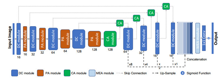
Accurate segmentation is a basic and crucial step for medical image processing and analysis. In the last few years, U-Net, and its variants, have become widely adopted models in medical image segmentation tasks. However, the multiple training parameters of these models determines high computation complexity, which is impractical for further applications. In this paper, by introducing depthwise separable convolution and attention mechanism into U-shaped architecture, we propose a novel lightweight neural network (DSCA-Net) for medical image segmentation. Three attention modules are created to improve its segmentation performance. Firstly, Pooling Attention (PA) module is utilized to reduce the loss of consecutive down-sampling operations. Secondly, for capturing critical context information, based on attention mechanism and convolution operation, we propose Context Attention (CA) module instead of concatenation operations. Finally, Multiscale Edge Attention (MEA) module is used to emphasize multi-level representative scale edge features for final prediction. The number of parameters in our network is 2.2 M, which is 71.6% less than U-Net. Experiment results across four public datasets show the potential and the dice coefficients are improved by 5.49% for ISIC 2018, 4.28% for thyroid, 1.61% for lung and 9.31% for nuclei compared with U-Net.

References

[1]	J. C. Caicedo, J. Roth, A. Goodman, T. Becker, K. W. Karhohs, M. Broisin, et al., Evaluation of deep learning strategies for nucleus segmentation in fluorescence images, Cytometry, Part A, J. Quant. Cell Sci., 95 (2019), 952–965. https://doi.org/10.1002/cyto.a.23863 doi: 10.1002/cyto.a.23863
[2]	Y. Fu, Y. Lei, T. Wang, W. J. Curran, T. Liu, X. Yang, A review of deep learning based methods for medical image multi-organ segmentation, Physica Med., 85 (2021), 107–122. https://doi.org/10.1016/j.ejmp.2021.05.003 doi: 10.1016/j.ejmp.2021.05.003
[3]	R. Merjulah, J. Chandra, Segmentation technique for medical image processing: a survey, in 2017 International Conference on Inventive Computing and Informatics (ICICI), (2017), 1055–1061. https://doi.org/10.1109/ICICI.2017.8365301
[4]	Z. Gu, J. Cheng, H. Fu, K. Zhou, H. Hao, Y. Zhao, et al., CE-Net: context encoder network for 2D medical image segmentation, IEEE Trans. Med. Imaging, 38 (2019), 2281–2292. https://doi.org/10.1109/TMI.2019.2903562 doi: 10.1109/TMI.2019.2903562
[5]	N. C. F. Codella, D. Gutman, M. E. Celebi, B. Helba, M. A. Marchetti, S. W. Dusza, et al., Skin lesion analysis toward melanoma detection: a challenge at the 2017 International symposium on biomedical imaging (ISBI), hosted by the international skin imaging collaboration (ISIC), in 2018 IEEE 15th International Symposium on Biomedical Imaging (ISBI 2018), (2018), 168–172. https://doi.org/10.1109/ISBI.2018.8363547
[6]	H. Yu, L. T. Yang, Q. Zhang, D. Armstrong, M. J. Deen, Convolutional neural networks for medical image analysis: state-of-the-art, comparisons, improvement and perspectives, Neurocomputing, 444 (2021), 92–110. https://doi.org/10.1016/j.neucom.2020.04.157 doi: 10.1016/j.neucom.2020.04.157
[7]	N. Tajbakhsh, L. Jeyaseelan, Q. Li, J. N. Chiang, Z. Wu, X. Ding, Embracing imperfect datasets: a review of deep learning solutions for medical image segmentation, Med. Image Anal., 63 (2020), 101693. https://doi.org/10.1016/j.media.2020.101693 doi: 10.1016/j.media.2020.101693
[8]	V. Badrinarayanan, A. Kendall, R. Cipolla, SegNet: a deep convolutional encoder-decoder architecture for image segmentation, IEEE Trans. Pattern Anal. Mach. Intell., 39 (2017), 2481–2495. https://doi.org/10.1109/TPAMI.2016.2644615 doi: 10.1109/TPAMI.2016.2644615
[9]	J. Long, E. Shelhamer, T. Darrell, Fully convolutional networks for semantic segmentation, in 2015 IEEE Conference on Computer Vision and Pattern Recognition (CVPR), (2015), 3431–3440. https://doi.org/10.1109/CVPR.2015.7298965
[10]	O. Ronneberger, P. Fischer, T. Brox, U-Net: convolutional networks for biomedical image segmentation, in Medical Image Computing and Computer-Assisted Intervention – MICCAI 2015, (2015), 234–241. https://doi.org/10.1007/978-3-319-24574-4_28
[11]	R. Gu, G. Wang, T. Song, R. Huang, M. Aertsen, J. Deprest, et al., CA-Net: comprehensive attention convolutional neural networks for explainable medical image segmentation, IEEE Trans. Med. Imaging, 40 (2021), 699–711. https://doi.org/10.1109/TMI.2020.3035253 doi: 10.1109/TMI.2020.3035253
[12]	N. Ibtehaz, M. S. Rahman, MultiResUNet: rethinking the U-Net architecture for multimodal biomedical image segmentation, Neural Networks, 121 (2020), 74–87. https://doi.org/10.1016/j.neunet.2019.08.025 doi: 10.1016/j.neunet.2019.08.025
[13]	C. Y. Chang, P. C. Chung, Y. C. Hong, C. H. Tseng, A neural network for thyroid segmentation and volume estimation in CT images, IEEE Comput. Intell. Mag., 6 (2011), 43–55. https://doi.org/10.1109/MCI.2011.942756 doi: 10.1109/MCI.2011.942756
[14]	S. Nandamuri, D. China, P. Mitra, D. Sheet, Sumnet: fully convolutional model for fast segmentation of anatomical structures in ultrasound volumes, in 2019 IEEE 16th International Symposium on Biomedical Imaging (ISBI 2019), (2019), 1729–1732. https://doi.org/10.1109/ISBI.2019.8759210
[15]	M. Z. Alom, C. Yakopcic, T. M. Taha, V. K. Asari, Recurrent residual convolutional neural network based on U-Net (R2U-Net) for medical image segmentation, in NAECON 2018 - IEEE National Aerospace and Electronics Conference, (2018), 228–233. https://doi.org/10.1109/NAECON.2018.8556686
[16]	Y. Wen, L. Chen, Y. Deng, J. Ning, C. Zhou, Towards better semantic consistency of 2D medical image segmentation, J. Visual Commun. Image Represent., 80 (2021), 103311. https://doi.org/10.1016/j.jvcir.2021.103311 doi: 10.1016/j.jvcir.2021.103311
[17]	P. Naylor, M. Lae, F. Reyal, T. Walter, Nuclei segmentation in histopathology images using deep neural networks, in 2017 IEEE 14th International Symposium on Biomedical Imaging (ISBI 2017), (2017), 933–936. https://doi.org/10.1109/ISBI.2017.7950669
[18]	H. Noh, S. Hong, B. Han, Learning deconvolution network for semantic segmentation, in 2015 IEEE International Conference on Computer Vision (ICCV), (2015), 1520–1528. https://doi.org/10.1109/ICCV.2015.178
[19]	Q. Kang, Q. Lao, T. Fevens, Nuclei segmentation in histopathological images using two-stage learning, in Medical Image Computing and Computer Assisted Intervention – MICCAI 2019, (2019), 703–711. https://doi.org/10.1007/978-3-030-32239-7_78
[20]	Z. Zhou, M. M. R. Siddiquee, N. Tajbakhsh, J. Liang, UNet++: a nested U-Net architecture for medical image segmentation, in Deep Learning in Medical Image Analysis and Multimodal Learning for Clinical Decision Support, 2018 (2018), 3–11. https://doi.org/10.1007/978-3-030-00889-5_1
[21]	L. Kaiser, A. N. Gomez, F. Chollet, Depthwise separable convolutions for neural machine translation, preprint, arXiv: 1706.03059.
[22]	J. Hu, L. Shen, G. Sun, Squeeze-and-excitation networks, in 2018 IEEE/CVF Conference on Computer Vision and Pattern Recognition, (2018), 7132–7141. https://doi.org/10.1109/CVPR.2018.00745
[23]	Q. Wang, B. Wu, P. Zhu, P. Li, W. Zuo, Q. Hu, ECA-Net: efficient channel attention for deep convolutional neural networks, in 2020 IEEE/CVF Conference on Computer Vision and Pattern Recognition (CVPR), (2020), 11531–11539. https://doi.org/10.1109/CVPR42600.2020.01155
[24]	V. Mnih, N. Heess, A. Graves, K. Kavukcuoglu, Recurrent models of visual attention, in Proceedings of the 27th International Conference on Neural Information Processing Systems, 2 (2014), 2204–2212. https://dl.acm.org/doi/abs/10.5555/2969033.2969073
[25]	D. Bahdanau, K. Cho, Y. Bengio, Neural machine translation by jointly learning to align and translate, preprint, arXiv: 1409.0473.
[26]	A. Vaswani, N. Shazeer, N. Parmar, J. Uszkoreit, L. Jones, A. N. Gomez, et al., Attention is all you need, in Advances in Neural Information Processing Systems, 30 (2017), 5998–6008. Available from: https://proceedings.neurips.cc/paper/2017/file/3f5ee243547dee91fbd053c1c4a845aa-Paper.pdf.
[27]	O. Oktay, J. Schlemper, L. L. Folgoc, M. Lee, M. Heinrich, K. Misawa, et al., Attention U-Net: learning where to look for the pancreas, preprint, arXiv: 1804.03999.
[28]	F. Chollet, Xception: deep learning with depthwise separable convolutions, in 2017 IEEE Conference on Computer Vision and Pattern Recognition (CVPR), (2017), 1800–1807. https://doi.org/10.1109/CVPR.2017.195
[29]	A. G. Howard, M. Zhu, B. Chen, D. Kalenichenko, W. Wang, T. Weyand, et al., Mobilenets: Efficient convolutional neural networks for mobile vision applications, preprint, arXiv: 1704.04861.
[30]	X. Zhang, X. Zhou, M. Lin, J. Sun, Shufflenet: an extremely efficient convolutional neural network for mobile devices, in 2018 IEEE/CVF Conference on Computer Vision and Pattern Recognition, (2018), 6848–6856. https://doi.org/10.1109/CVPR.2018.00716
[31]	L. C. Chen, Y. Zhu, G. Papandreou, F. Schroff, H. Adam, Encoder-decoder with atrous separable convolution for semantic image segmentation, in Computer Vision – ECCV 2018, (2018), 833–851. https://doi.org/10.1007/978-3-030-01234-2_49
[32]	K. Qi, H. Yang, C. Li, Z. Liu, M. Wang, Q. Liu, et al., X-Net: brain stroke lesion segmentation based on depthwise separable convolution and long-range dependencies, in Medical Image Computing and Computer Assisted Intervention – MICCAI 2019, (2019), 247–255.https://doi.org/10.1007/978-3-030-32248-9_28
[33]	A. Wibowo, S. R. Purnama, P. W. Wirawan, H. Rasyidi, Lightweight encoder-decoder model for automatic skin lesion segmentation, Inf. Med. Unlocked, 25 (2021), 100640. https://doi.org/10.1016/j.imu.2021.100640 doi: 10.1016/j.imu.2021.100640
[34]	C. Meng, K. Sun, S. Guan, Q. Wang, R. Zong, L. Liu, Multiscale dense convolutional neural network for DSA cerebrovascular segmentation, Neurocomputing, 373 (2020), 123–134. https://doi.org/10.1016/j.neucom.2019.10.035 doi: 10.1016/j.neucom.2019.10.035
[35]	G. Huang, Z. Liu, L. V. D. Maaten, K. Q. Weinberger, Densely connected convolutional networks, in 2017 IEEE Conference on Computer Vision and Pattern Recognition (CVPR), (2017), 2261–2269. https://doi.org/10.1109/CVPR.2017.243
[36]	Y. Wu, K. He, Group normalization, Int. J. Comput. Vision, 128 (2020), 742–755. https://doi.org/10.1007/s11263-019-01198-w doi: 10.1007/s11263-019-01198-w
[37]	X. Zhang, Y. Zou, W. Shi, Dilated convolution neural network with LeakyReLU for environmental sound classification, in 2017 22nd International Conference on Digital Signal Processing (DSP), (2017), 1–5. https://doi.org/10.1109/ICDSP.2017.8096153
[38]	P. Tschandl, C. Rosendahl, H. Kittler, The HAM10000 dataset, a large collection of multi-source dermatoscopic images of common pigmented skin lesions, Sci. Data, 5 (2018), 180161. https://doi.org/10.1038/sdata.2018.161 doi: 10.1038/sdata.2018.161
[39]	T. Wunderling, B. Golla, P. Poudel, C. Arens, M. Friebe, C. Hansen, Comparison of thyroid segmentation techniques for 3D ultrasound, Med. Imaging 2017: Image Process., 10133 (2017), 1013317. https://doi.org/10.1117/12.2254234 doi: 10.1117/12.2254234
[40]	D. P. Kingma, J. Ba, Adam: a method for stochastic optimization, preprint, arXiv: 1412.6980.
[41]	G. Lin, A. Milan, C. Shen, I. Reid, RefineNet: Multi-path refinement networks for high-resolution semantic segmentation, in 2017 IEEE Conference on Computer Vision and Pattern Recognition (CVPR), (2017), 5168–5177. https://doi.org/10.1109/CVPR.2017.549
[42]	R. Ma, S. Zhang, C. Gan, H. Zhao, EOCNet: Improving edge omni-scale convolution networks for skin lesion segmentation, in 2020 3rd International Conference on Digital Medicine and Image Processing, (2020), 45–50. https://doi.org/10.1145/3441369.3441377
[43]	L. C. Chen, G. Papandreou, I. Kokkinos, K. Murphy, A. L. Yuille, DeepLab: Semantic image segmentation with deep convolutional nets, atrous convolution, and fully connected CRFs, IEEE Trans. Pattern Anal. Mach. Intell., 40 (2018), 834–848. https://doi.org/10.1109/TPAMI.2017.2699184 doi: 10.1109/TPAMI.2017.2699184
[44]	S. Chen, Y. Zou, P. X. Liu, IBA-U-Net: Attentive BConvLSTM U-Net with redesigned inception for medical image segmentation, Comput. Biol. Med., 135 (2021), 104551. https://doi.org/10.1016/j.compbiomed.2021.104551 doi: 10.1016/j.compbiomed.2021.104551

Reader Comments

Your name:*

Email:*
© 2023 the Author(s), licensee AIMS Press. This is an open access article distributed under the terms of the Creative Commons Attribution License (http://creativecommons.org/licenses/by/4.0)