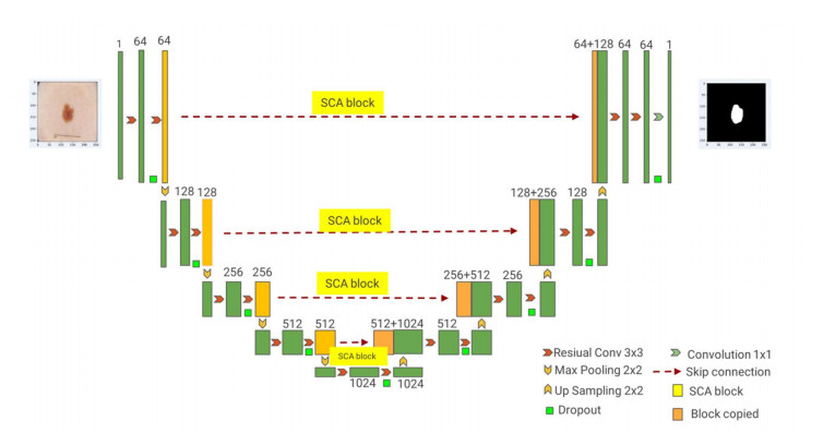
For the problems of blurred edges, uneven background distribution, and many noise interferences in medical image segmentation, we proposed a medical image segmentation algorithm based on deep neural network technology, which adopts a similar U-Net backbone structure and includes two parts: encoding and decoding. Firstly, the images are passed through the encoder path with residual and convolutional structures for image feature information extraction. We added the attention mechanism module to the network jump connection to address the problems of redundant network channel dimensions and low spatial perception of complex lesions. Finally, the medical image segmentation results are obtained using the decoder path with residual and convolutional structures. To verify the validity of the model in this paper, we conducted the corresponding comparative experimental analysis, and the experimental results show that the DICE and IOU of the proposed model are 0.7826, 0.9683, 0.8904, 0.8069, and 0.9462, 0.9537 for DRIVE, ISIC2018 and COVID-19 CT datasets, respectively. The segmentation accuracy is effectively improved for medical images with complex shapes and adhesions between lesions and normal tissues.
Citation: Tongping Shen, Fangliang Huang, Xusong Zhang. CT medical image segmentation algorithm based on deep learning technology[J]. Mathematical Biosciences and Engineering, 2023, 20(6): 10954-10976. doi: 10.3934/mbe.2023485
For the problems of blurred edges, uneven background distribution, and many noise interferences in medical image segmentation, we proposed a medical image segmentation algorithm based on deep neural network technology, which adopts a similar U-Net backbone structure and includes two parts: encoding and decoding. Firstly, the images are passed through the encoder path with residual and convolutional structures for image feature information extraction. We added the attention mechanism module to the network jump connection to address the problems of redundant network channel dimensions and low spatial perception of complex lesions. Finally, the medical image segmentation results are obtained using the decoder path with residual and convolutional structures. To verify the validity of the model in this paper, we conducted the corresponding comparative experimental analysis, and the experimental results show that the DICE and IOU of the proposed model are 0.7826, 0.9683, 0.8904, 0.8069, and 0.9462, 0.9537 for DRIVE, ISIC2018 and COVID-19 CT datasets, respectively. The segmentation accuracy is effectively improved for medical images with complex shapes and adhesions between lesions and normal tissues.

| [1] | J. Chen, Y. Lu, Q. Yu, X. Luo, E. Adeli, Y. Wang, et al., TransUNet: Transformers make strong encoders for medical image segmentation, preprint, arXiv: 2102.04306. |
| [2] |
T. P. Shen, H. Q. Xu, Medical image segmentation based on Transformer and HarDNet structures, IEEE Access, 11 (2023), 16621–16630. https://doi.org/10.1109/ACCESS.2023.3244197 doi: 10.1109/ACCESS.2023.3244197

|
| [3] |
L. Han, Y. H. Chen, J. M. Li, B. W. Zhong, Y. Z. Lei, M. H. Sun, Liver segmentation with 2.5 D perpendicular UNets, Comput. Electr. Eng., 91 (2021), 107118. https://doi.org/10.1016/j.compeleceng.2021.107118 doi: 10.1016/j.compeleceng.2021.107118
|
| [4] |
H. Y. Li, X. Q. Zhao, A. Y. Su, H. T. Zhang, J. X. Liu, G. Y. Gu, Color space transformation and multi-class weighted loss for adhesive white blood cell segmentation, IEEE Access, 8 (2020), 24808–24818. https://doi.org/10.1109/ACCESS.2020.2970485 doi: 10.1109/ACCESS.2020.2970485
|
| [5] |
T. Magadza, S. Viriri, Deep learning for brain tumor segmentation: a survey of state-of-the-art, J. Imaging, 7 (2021), 19. https://doi.org/10.3390/jimaging7020019 doi: 10.3390/jimaging7020019
|
| [6] |
Y. E. Almalki, A. Qayyum, M. Irfan, N. Haider, A. Glowacz, F. M. Alshehri, et al., A novel method for COVID-19 diagnosis using artificial intelligence in chest X-ray images, Healthcare, 9 (2021), 522. https://doi.org/10.3390/healthcare9050522 doi: 10.3390/healthcare9050522
|
| [7] |
D. Q. Zhang, S. C. Chen, A novel kernelized fuzzy c-means algorithm with application in medical image segmentation, Artif. Intell. Med., 32 (2014), 37–50. https://doi.org/10.1016/j.artmed.2004.01.012 doi: 10.1016/j.artmed.2004.01.012
|
| [8] | H. P. Ng, S. H. Ong, K. W. C. Foong, Poh-Sun Goh, W. L. Nowinski, Medical image segmentation using k-means clustering and improved watershed algorithm, in 2006 IEEE southwest symposium on image analysis and interpretation, (2006). https://doi.org/10.1109/SSIAI.2006.1633722 |
| [9] | N. A. Mohamed, M. N. Ahmed, A. Farag, Modified fuzzy c-mean in medical image segmentation, in 1999 IEEE International Conference on Acoustics, (1999). https://doi.org/10.1109/ICASSP.1999.757579 |
| [10] | A. Prabin A, J. Veerappan, Automatic segmentation of lung ct images by CC based region growing, J. Theor. Appl. Inf. Technol., 68 (2014), 63–69. |
| [11] |
M. Negassi, R. Suarez-Ibarrola, S. Hein, A. Miernik, A. Reiterer, Application of artificial neural networks for automated analysis of cystoscopic images: a review of the current status and future prospects, World J. Urol., 38 (2020), 2349–2358. https://doi.org/10.1007/s00345-019-03059-0 doi: 10.1007/s00345-019-03059-0
|
| [12] |
Y. Zhang, M. A. Khan, Z. Zhu, S. Wang, SNELM: SqueezeNet-guided ELM for COVID-19 recognition, Comput. Syst. Sci. Eng., 46 (2023), 13–26. https://doi.org/10.32604/csse.2023.034172 doi: 10.32604/csse.2023.034172
|
| [13] |
M. Irfan, M. A. Iftikhar, S. Yasin, U. Draz, T. Ali, S. Hussain, et al., Role of hybrid deep neural networks (HDNNs), computed tomography, and chest X-rays for the detection of COVID-19, Int. J. Environ. Res. Public Health, 18 (2021), 3056. https://doi.org/10.3390/ijerph18063056 doi: 10.3390/ijerph18063056
|
| [14] | J. Long, E. Shelhamer, T. Darrell, Fully convolutional networks for semantic segmentation, in Proceedings of the 2015 IEEE Conference on Computer Vision and Pattern Recognition, (2015). https://doi.org/10.1109/CVPR.2015.7298965 |
| [15] | O. Ronneberger, P. Fischer, T. Brox, U-net: Convolutional networks for biomedical image segmentation, in International Conference on Medical image computing and computer-assisted intervention, (2015). https://doi.org/10.1007/978-3-319-24574-4_28 |
| [16] |
Z. W. Zhou, M. M. R. Siddiquee, N. Tajbakhsh, J. M. Liang, Unet++: redesigning skip connections to exploit multiscale features in image segmentation, IEEE Trans. Med. Imaging, 39 (2020), 1856–1867. https://doi.org/10.1109/TMI.2019.2959609 doi: 10.1109/TMI.2019.2959609
|
| [17] | O. Oktay, J. Schlemper, L. L. Folgoc, M. Lee, M. Heinrich, K. Misawa, et al., Attention U-Net: learning where to look for the Pancreas, preprint, arXiv: 1804.03999. |
| [18] |
D. L. Peng, S. Y. Xiong, W. J. Peng, J. P. Lu, LCP-net: a local context-perception deep neural network for medical image segmentation, Expert Syst. Appl., 168 (2021), 114234. https://doi.org/10.1016/j.eswa.2020.114234 doi: 10.1016/j.eswa.2020.114234
|
| [19] |
C. Chen, B. Liu, K. N. Zhou, W. Z. He, F. Yan, Z. L. Wang, R. X. Xiao, CSR-net: cross-scale residual network for multi- objective scaphoid fracture segmentation, Comput. Biol. Med., 137 (2021), 104776. https://doi.org/10.1016/j.compbiomed.2021.104776 doi: 10.1016/j.compbiomed.2021.104776
|
| [20] |
E. K. Wang, C. M. Chen, M. M. Hassan, A. Almogren, A deep learning based medical image segmentation technique in Internet-of-Medical-Things domain, Future Gene. Comput. Sy., 108 (2020), 135–144. https://doi.org/10.1016/j.future.2020.02.054 doi: 10.1016/j.future.2020.02.054
|
| [21] |
T. Feng, C. S. Wang, X. W. Chen, H. T. Fan, K. Zeng, Z. Y. Li, URNet: A UNet based residual network for image dehazing, Appl. Soft Comput., 102 (2020), 106884. https://doi.org/10.1016/j.asoc.2020.106884 doi: 10.1016/j.asoc.2020.106884
|
| [22] |
R. Q. Ge, H. H. Cai, X. Yuan, F. W. Qin, Y. Huang, et al., MD-UNET: Multiinput dilated U-shape neural network for segmentation of bladder cancer, Comput. Biol. Chem., 93 (2021), 107510. https://doi.org/10.1016/j.compbiolchem.2021.107510 doi: 10.1016/j.compbiolchem.2021.107510
|
| [23] |
Y. C. Lan, X. M. Zhang, Real-time ultrasound image despeckling using mixed-attention mechanism based residual UNet, IEEE Access, 8 (2020), 195327–195340. https://doi.org/10.1109/ACCESS.2020.3034230 doi: 10.1109/ACCESS.2020.3034230
|
| [24] |
C. Li, Y. S. Tan, W. Chen, X. Luo, Y. L. He, Y. M. Gao, F. Li, ANU-Net: Attention-based nested U-Net to exploit full resolution features for medical image segmentation, Comput. Graph, 90 (2020), 11–20. https://doi.org/10.1016/j.cag.2020.05.003 doi: 10.1016/j.cag.2020.05.003
|
| [25] | C. L. Guo, M. Szemenyei, Y. G. Yi, W. L. Wang, B. Chen, C. Q. Fan, SA-UNet: Spatial attention U-Net for retinal vessel segmentation, in 25th International Conference on Pattern Recognition (ICPR), (2021). https://doi.org/10.1109/ICPR48806.2021.9413346 |
| [26] |
J. Bernal, F. J. Sánchez, G. Fernández-Esparrach, D. Gil, C. Rodríguez, F. Vilariño, WM-DOVA maps for accurate polyp highlighting in colonoscopy: validation vs. saliency maps from physicians, Comput. Med. Imaging Graphics, 43 (2015), 99–111. https://doi.org/10.1016/j.compmedimag.2015.02.007 doi: 10.1016/j.compmedimag.2015.02.007
|
| [27] |
J. Soltani-Nabipour, A. Khorshidi, B. Noorian, Lung tumor segmentation using improved region growing algorithm, Nuclear Eng. Technol., 52 (2020), 2313–2319. https://doi.org/10.1016/j.net.2020.03.011 doi: 10.1016/j.net.2020.03.011
|
| [28] | S. Y. Chong, M. K. Tan, K. B. Yeo, M. Y. Ibrahim, X. Hao, K. T. K. Teo, Segmenting nodules of lung tomography image with level set algorithm and neural network, in 2019 IEEE 7th Conference on Systems, Process and Control (ICSPC), (2019). https://doi.org/10.1109/ICSPC47137.2019.9067987 |
| [29] |
M. Savic, Y. Ma, G. Ramponi, W. Du, Y. Peng, Lung nodule segmentation with a region-based fast marching method, Sensors, 21 (2021), 1908. https://doi.org/10.3390/s21051908 doi: 10.3390/s21051908
|
| [30] | P. M. Bruntha, S. I. A. Pandian, P. Mohan, Active Contour Model (without edges) based pulmonary nodule detection in low dose CT images, in 2019 2nd International Conference on Signal Processing and Communication (ICSPC), (2019). https://doi.org/10.1109/ICSPC46172.2019.8976813 |
| [31] | R. Manickavasagam, S. Selvan, GACM based segmentation method for Lung nodule detection and classification of stages using CT images, in 2019 1st International Conference on Innovations in Information and Communication Technology (ICIICT), (2019). https://doi.org/10.1109/ICIICT1.2019.8741477. |
| [32] |
Y. LeCun, L. Bottou, Y. Bengio, P. Haffner, Gradient-based learning applied to document recognition, Proc. IEEE, 86 (1998), 2278–2324. https://doi.org/10.1109/5.726791 doi: 10.1109/5.726791
|
| [33] |
G. Simantiris, G. Tziritas, Cardiac MRI segmentation with a dilated CNN incorporating domain-specific constraints, IEEE J. Selected Topics Signal Process., 14 (2020), 1235–1243. https://doi.org/10.1109/JSTSP.2020.3013351 doi: 10.1109/JSTSP.2020.3013351
|
| [34] |
B. Thyreau, Y. Taki, Learning a cortical parcellation of the brain robust to the MRI segmentation with convolutional neural networks, Med. Image Anal., 14 (2020), 101639. https://doi.org/10.1016/j.media.2020.101639 doi: 10.1016/j.media.2020.101639
|
| [35] |
M. F. Aslan, A robust semantic lung segmentation study for CNN-based COVID-19 diagnosis, Chemom. Intell. Lab. Syst., 231 (2022), 104695. https://doi.org/10.1016/j.chemolab.2022.104695 doi: 10.1016/j.chemolab.2022.104695
|
| [36] |
S. Akila Agnes, J. Anitha, J. D. Peter, Automatic lung segmentation in low-dose chest CT scans using convolutional deep and wide network (CDWN), Neural Comput. Appl., 32 (2020), 15845-15855. https://doi.org/10.1007/s00521-018-3877-3 doi: 10.1007/s00521-018-3877-3
|
| [37] |
L. L. Du, H. R. Liu, L. Zhang, Y. Lu, M. Y. Li, Y. Hu, et al., Deep ensemble learning for accurate retinal vessel segmentation, Comput. Biol. Med., 158 (2023), 106829. https://doi.org/10.1016/j.compbiomed.2023.106829 doi: 10.1016/j.compbiomed.2023.106829
|
| [38] |
Y. Wu, L. Lin, Automatic lung segmentation in CT images using dilated convolution based weighted fully convolutional network, J. Phys. Confer. Ser., 1646 (2022), 012032. https://doi.org/10.1088/1742-6596/1646/1/012032 doi: 10.1088/1742-6596/1646/1/012032
|
| [39] |
H. Xia, W. Sun, S. Song, X. Mou, Md-net: multi-scale dilated convolution network for CT images segmentation, Neural Process. Lett., 51 (2020), 2915–2927. https://doi.org/10.1007/s11063-020-10230-x doi: 10.1007/s11063-020-10230-x
|
| [40] |
H. Liu, H. Cao, E. Song, G. Ma, X. Xu, R. Jin, C. C. Hung, A cascaded dual-pathway residual network for lung nodule segmentation in CT images, Phys. Med., 63 (2019), 112–121. https://doi.org/10.1016/j.ejmp.2019.06.003 doi: 10.1016/j.ejmp.2019.06.003
|
| [41] |
H. R. Roth, H. Oda, X. Zhou, N. Shimizu, Y. Yang, Y. Hayash, et al., An application of cascaded 3D fully convolutional networks for medical image segmentation, Comput. Med. Imaging Graphics, 66 (2018), 90–99. https://doi.org/10.1016/j.compmedimag.2018.03.001 doi: 10.1016/j.compmedimag.2018.03.001
|
| [42] |
A. Lin, B. Chen, J. Xu, Z. Zhang, G. Lu, D. Zhang, Ds-transunet: Dual swin transformer u-net for medical image segmentation, IEEE Trans. Instrum. Meas., 71 (2022), 1–15. https://doi.org/10.1109/TIM.2022.3178991 doi: 10.1109/TIM.2022.3178991
|
| [43] | F. Milletari, N. Navab, S. A. Ahmadi, V-net: Fully convolutional neural networks for volumetric medical image segmentation, in 2016 Fourth International Conference on 3D Vision (3DV), (2016). https://doi.org/10.48550/arXiv.1606.04797 |
| [44] |
F. Hoorali, H. Khosravi, B. Moradi, IRUNet for medical image segmentation, Expert Syst. Appl., 191 (2022), 116399. https://doi.org/10.1016/j.eswa.2021.116399 doi: 10.1016/j.eswa.2021.116399
|
| [45] | H. Huang, L. Lin, R. Tong, H. Hu, Q. Zhang, Y. Iwamoto, et al., UNet 3+: A full-scale connected UNet for medical image segmentation, in 2020 IEEE International Conference on Acoustics, Speech and Signal Processing, (2020). https://doi.org/10.48550/arXiv.2004.08790 |
| [46] |
M. Z. Alom, C. Yakopcic, T. M. Taha, V. K. Asari, Nuclei segmentation with recurrent residual convolutional neural networks based U-net(R2U-net), 2018-IEEE National Aerospace and Electronics Conference, (2018). https://doi.org/10.1109/NAECON.2018.8556686 doi: 10.1109/NAECON.2018.8556686
|
| [47] |
T. Shen, X. G. Li, Automatic polyp image segmentation and cancer prediction based on deep learning, Front. Oncol., 12 (2022), 1087438. https://doi.org/10.3389/fonc.2022.1087438 doi: 10.3389/fonc.2022.1087438
|
| [48] |
Z. Han, M. Jian, G. G. Wang, ConvUNeXt: An efficient convolution neural network for medical image segmentation, Knowl. Based Syst., 253 (2022), 109512. https://doi.org/10.1016/j.knosys.2022.109512 doi: 10.1016/j.knosys.2022.109512
|
| [49] |
R. Gu, G. Wang, T. Song, R. Huang, M. Aertsen, J. Deprest, et al., CA-Net: Comprehensive attention convolutional neural networks for explainable medical image segmentation, IEEE Trans. Med. Imaging, 40 (2020), 699–711. https://doi.org/10.48550/arXiv.2009.10549 doi: 10.48550/arXiv.2009.10549
|
| [50] |
J. Zhang, X. Lv, H. Zhang, B. Liu, AResU-Net: Attention residual U-Net for brain tumor segmentation, Symmetry, 12 (2020), 721. https://doi.org/10.3390/sym12050721 doi: 10.3390/sym12050721
|
| [51] |
X. Tong, J. Wei, B. Sun, S. Su, Z. Zuo, P. Wu, ASCU-Net: attention gate, spatial and channel attention u-net for skin lesion segmentation, Diagnostics, 11 (2021), 501. https://doi.org/10.3390/diagnostics11030501 doi: 10.3390/diagnostics11030501
|
| [52] | J. Fu, J. Liu, H. J. Tian, Y. Li, Y. J. Bao, Z. W. Fang, et al., Dual attention network for scene segmentation, in Proceedings of the IEEE/CVF conference on computer vision and pattern recognition, (2019). https://doi.org/10.48550/arXiv.1809.02983 |
| [53] |
K. M. He, X. Y. Zhang, S. Q. Ren, J. Sun, Deep residual learning for image recognition, Proceedings of the IEEE Conference on Computer Vision and Pattern Recognition (CVPR), (2016). https://doi.org/10.1109/CVPR.2016.90 doi: 10.1109/CVPR.2016.90
|
| [54] |
M. Jun, J. N. Chen, M. Ng, R. Huang, Y. Li, C. Li, et al., Loss odyssey in medical image segmentation, Med. Image Anal., 71 (2021), 102035. https://doi.org/10.1016/j.media.2021.102035 doi: 10.1016/j.media.2021.102035
|
| [55] |
R. Wang, T. Lei, R. Cui, B. Zhang, H. Meng, A. K. Nandi, Medical image segmentation using deep learning: a survey, IET Image Process., 162 (2022), 1243–1267. https://doi.org/10.48550/arXiv.2009.13120 doi: 10.48550/arXiv.2009.13120
|
| [56] | T. Y. Lin, P. Goyal, R. Girshick, K. He, P. Dollár, Focal loss for dense object detection, in Proceedings of the IEEE international conference on computer vision, (2017). https://doi.org/10.48550/arXiv.1708.02002 |
| [57] | N. Codella, V. Rotemberg, P. Tschandl, M. E. Celebi, S. Dusza, D. Gutman, et al., Skin lesion analysis toward melanoma detection 2018: A challenge hosted by the international skin imaging collaboration (isic), preprint, arXiv: 1902.03368. |
| [58] | M. Yahyatabar, P. Jouvet, F. Cheriet, Dense-Unet: a light model for lung fields segmentation in Chest X-Ray images, in 42nd Annual International Conference of the IEEE Engineering in Medicine & Biology Society (EMBC), (2020). https://doi.org/10.1109/EMBC44109.2020.9176033 |
| [59] |
Y. Sun, F. K. Bi, Y. T. Gao, L. Chen, S. T. Feng, A Multi-Attention UNet for Semantic Segmentation in Remote Sensing Images, Symmetry, 14 (2022), 906. https://doi.org/10.3390/sym14050906 doi: 10.3390/sym14050906
|
| [60] |
Q. Jin, Z. Meng, T. D. Pham, Q. Chen, L. Wei, R. Su, Dunet: A deformable network for retinal vessel segmentation, Knowledge-Based Systems, 178 (2018), 149–162. https://doi.org/10.48550/arXiv.1811.01206 doi: 10.48550/arXiv.1811.01206
|
| [61] | L. Li, M. Verma, Y. Nakashima, H. Nagahara, R. Kawasaki, Iternet: Retinal image segmentation utilizing structural redundancy in vessel networks, in The IEEE Winter Conference on Applications of Computer Vision, (2020). https://doi.org/10.1109/WACV45572.2020.9093621 |
| [62] | S. A. Kamran, K. F. Hossain, A. Tavakkoli, S. L. Zuckerbrod, K. M. Sanders, S. A. Baker, RV-GAN: segmenting retinal vascular structure in fundus photographs using a novel multi-scale generative adversarial network, in International Conference on Medical Image Computing and Computer-Assisted Intervention, (2021). https://doi.org/10.48550/arXiv.2101.00535 |
| [63] | Y. Zhang, H. Liu, Q. Hu, Transfuse: Fusing transformers and cnns for medical image segmentation, in International Conference on Medical Image Computing and Computer-Assisted Intervention, (2021). https://doi.org/10.48550/arXiv.2102.08005 |
| [64] | J. Wei, Y. Hu, R. Zhang, Z. Li, S. K. Zhou, S. Cui, Shallow attention network for polyp segmentation, in International Conference on Medical Image Computing and Computer-Assisted Intervention, (2021). https://doi.org/10.48550/arXiv.2108.00882 |
| [65] | J. M. J. Valanarasu, V. M. Patel, Unext: Mlp-based rapid medical image segmentation network, preprint, arXiv: 2203.04967. |
| [66] | R. Azad, M. Asadi-Aghbolaghi, M. Fathy, S. Escalera, Bi-directional ConvLSTM U-Net with densley connected convolutions, in Proceedings of the IEEE/CVF international conference on computer vision workshops, (2019). https://doi.org/10.48550/arXiv.1909.00166 |
| [67] | X. G. Peng, D. L. Peng, MDA-Net: a medical image segmentation network combining dual-path attention mechanism, Small Microcomputer Syst., 43 (2022), 1–9. http://kns.cnki.net/kcms/detail/21.1106.tp.20220729.1534.034.html. |


Figures(11) / Tables(4)

Tongping Shen, Fangliang Huang, Xusong Zhang. CT medical image segmentation algorithm based on deep learning technology[J]. Mathematical Biosciences and Engineering, 2023, 20(6): 10954-10976. doi: 10.3934/mbe.2023485


 DownLoad: