In this paper, we construct the SV1V2EIR model to reveal the impact of two-dose vaccination on COVID-19 by using Caputo fractional derivative. The feasibility region of the proposed model and equilibrium points is derived. The basic reproduction number of the model is derived by using the next-generation matrix method. The local and global stability analysis is performed for both the disease-free and endemic equilibrium states. The present model is validated using real data reported for COVID-19 cumulative cases for the Republic of India from 1 January 2022 to 30 April 2022. Next, we conduct the sensitivity analysis to examine the effects of model parameters that affect the basic reproduction number. The Laplace Adomian decomposition method (LADM) is implemented to obtain an approximate solution. Finally, the graphical results are presented to examine the impact of the first dose of vaccine, the second dose of vaccine, disease transmission rate, and Caputo fractional derivatives to support our theoretical results.
Citation: Hardik Joshi, Brajesh Kumar Jha, Mehmet Yavuz. Modelling and analysis of fractional-order vaccination model for control of COVID-19 outbreak using real data[J]. Mathematical Biosciences and Engineering, 2023, 20(1): 213-240. doi: 10.3934/mbe.2023010
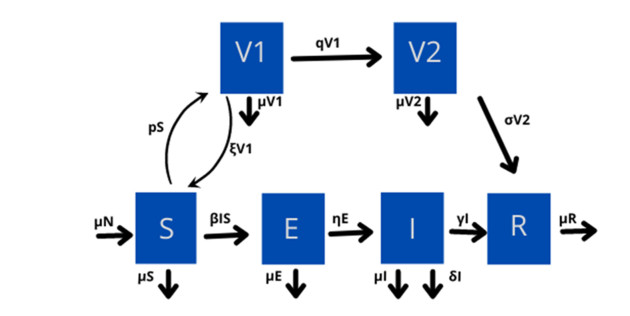
In this paper, we construct the SV1V2EIR model to reveal the impact of two-dose vaccination on COVID-19 by using Caputo fractional derivative. The feasibility region of the proposed model and equilibrium points is derived. The basic reproduction number of the model is derived by using the next-generation matrix method. The local and global stability analysis is performed for both the disease-free and endemic equilibrium states. The present model is validated using real data reported for COVID-19 cumulative cases for the Republic of India from 1 January 2022 to 30 April 2022. Next, we conduct the sensitivity analysis to examine the effects of model parameters that affect the basic reproduction number. The Laplace Adomian decomposition method (LADM) is implemented to obtain an approximate solution. Finally, the graphical results are presented to examine the impact of the first dose of vaccine, the second dose of vaccine, disease transmission rate, and Caputo fractional derivatives to support our theoretical results.

| [1] |
P. A. Naik, K. M. Owolabi, J. Zu, M. U. D. Naik, Modeling the transmission dynamics of COVID-19 pandemic in caputo type fractional derivative, J. Multiscale Model., 12 (2021). https://doi.org/10.1142/S1756973721500062 doi: 10.1142/S1756973721500062

|
| [2] |
K. M. Safare, V. S. Betageri, D. G. Prakasha, P. Veeresha, S. Kumar, A mathematical analysis of ongoing outbreak COVID-19 in India through nonsingular derivative, Numer. Meth. Part. Differ. Equations., 37 (2021), 1282–1298. https://doi.org/10.1002/num.22579 doi: 10.1002/num.22579
|
| [3] |
K. S. Nisar, S. Ahmad, A. Ullah, K. Shah, H. Alrabaiah, M. Arfan, Mathematical analysis of SIRD model of COVID-19 with Caputo fractional derivative based on real data, Results Phys., 21 (2021), 103772. https://doi.org/10.1016/j.rinp.2020.103772 doi: 10.1016/j.rinp.2020.103772
|
| [4] |
P. A. Naik, M. Yavuz, S. Qureshi, J. Zu, S. Townley, Modeling and analysis of COVID-19 epidemics with treatment in fractional derivatives using real data from Pakistan, Eur. Phys. J. Plus, 135 (2020), 795. https://doi.org/10.1140/epjp/s13360-020-00819-5 doi: 10.1140/epjp/s13360-020-00819-5
|
| [5] |
F. Özköse, M. Yavuz, Investigation of interactions between COVID-19 and diabetes with hereditary traits using real data: A case study in Turkey, Comput. Biol. Med., 141 (2022), 105044. https://doi.org/10.1016/j.compbiomed.2021.105044 doi: 10.1016/j.compbiomed.2021.105044
|
| [6] |
P. Pandey, J. F. Gómez-Aguilar, M. K. A. Kaabar, Z. Siri, A. A. A. Mousa, Mathematical modeling of COVID-19 pandemic in India using Caputo-Fabrizio fractional derivative, Comput. Biol. Med., 145 (2022), 105518. https://doi.org/10.1016/j.compbiomed.2022.105518 doi: 10.1016/j.compbiomed.2022.105518
|
| [7] |
N. Sene, Analysis of the stochastic model for predicting the novel coronavirus disease, Adv. Differ. Equations, 568 (2020), 1–19. https://doi.org/10.1186/s13662-020-03025-w doi: 10.1186/s13662-020-03025-w
|
| [8] |
T. Sitthiwirattham, A. Zeb, S. Chasreechai, Z. Eskandari, M. Tilioua, S. Djilali, Analysis of a discrete mathematical COVID-19 model, Results Phys., 28 (2021), 104668. https://doi.org/10.1016/j.rinp.2021.104668 doi: 10.1016/j.rinp.2021.104668
|
| [9] |
S. Kumar, R. P. Chauhan, S. Momani, S. Hadid, Numerical investigations on COVID-19 model through singular and non-singular fractional operators, Numer. Methods Partial Differ. Equations, (2020), 1–27. https://doi.org/10.1002/num.22707 doi: 10.1002/num.22707
|
| [10] |
F. Özköse, M. Yavuz, M. T. Şenel, R. Habbireeh, Fractional order modelling of omicron SARS-CoV-2 variant containing heart attack effect using real data from the United Kingdom, Chaos Solitons Fractals, 157 (2022), 111954. https://doi.org/10.1016/j.chaos.2022.111954 doi: 10.1016/j.chaos.2022.111954
|
| [11] |
A. Atangana, Modelling the spread of COVID-19 with new fractal-fractional operators: Can the lockdown save mankind before vaccination?, Chaos Solitons Fractals, 136 (2020), 109860. https://doi.org/10.1016/j.chaos.2020.109860 doi: 10.1016/j.chaos.2020.109860
|
| [12] |
T. Sardar, S. S. Nadim, S. Rana, J. Chattopadhyay, Assessment of lockdown effect in some states and overall India: A predictive mathematical study on COVID-19 outbreak, Chaos Solitons Fractals, 139 (2020), 110078. https://doi.org/10.1016/j.chaos.2020.110078 doi: 10.1016/j.chaos.2020.110078
|
| [13] | S. Choi, M. Ki, Analyzing the effects of social distancing on the COVID-19 pandemic in Korea using mathematical modeling, Epidemiol. Health, 42 (2020). https://doi.org/10.4178/epih.e2020064 |
| [14] |
D. Aldila, S. H. A. Khoshnaw, E. Safitri, Y. R. Anwar, A. R. Q. Bakry, B. M. Samiadji, et al., A mathematical study on the spread of COVID-19 considering social distancing and rapid assessment: The case of Jakarta, Indonesia, Chaos Solitons Fractals, 139 (2020), 110042. https://doi.org/10.1016/j.chaos.2020.110042 doi: 10.1016/j.chaos.2020.110042
|
| [15] |
D. Baleanu, M. Hassan Abadi, A. Jajarmi, K. Zarghami Vahid, J. J. Nieto, A new comparative study on the general fractional model of COVID-19 with isolation and quarantine effects, Alex. Eng. J., 61 (2022), 4779–4791. https://doi.org/10.1016/j.aej.2021.10.030 doi: 10.1016/j.aej.2021.10.030
|
| [16] |
Z. Memon, S. Qureshi, B. R. Memon, Assessing the role of quarantine and isolation as control strategies for COVID-19 outbreak: A case study, Chaos Solitons Fractals, 144 (2021), 110655. https://doi.org/10.1016/j.chaos.2021.110655 doi: 10.1016/j.chaos.2021.110655
|
| [17] |
A. M. Mishra, S. D. Purohit, K. M. Owolabi, Y. D. Sharma, A nonlinear epidemiological model considering asymptotic and quarantine classes for SARS CoV-2 virus, Chaos Solitons Fractals, 138 (2020), 109953. https://doi.org/10.1016/j.chaos.2020.109953 doi: 10.1016/j.chaos.2020.109953
|
| [18] |
A. Din, A. Khan, D. Baleanu, Stationary distribution and extinction of stochastic coronavirus (COVID-19) epidemic model, Chaos Solitons Fractals, 139 (2020), 110036. https://doi.org/10.1016/j.chaos.2020.110036 doi: 10.1016/j.chaos.2020.110036
|
| [19] |
P. Pandey, Y. M. Chu, J. F. Gómez-Aguilar, H. Jahanshahi, A. A. Aly, A novel fractional mathematical model of COVID-19 epidemic considering quarantine and latent time, Results Phys., 26 (2021), 104286. https://doi.org/10.1016/j.rinp.2021.104286 doi: 10.1016/j.rinp.2021.104286
|
| [20] |
Y. Gu, S. Ullah, M. A. Khan, M. Y. Alshahrani, M. Abohassan, M. B. Riaz, Mathematical modeling and stability analysis of the COVID-19 with quarantine and isolation, Results Phys., 34 (2022), 105284. https://doi.org/10.1016/j.rinp.2022.105284 doi: 10.1016/j.rinp.2022.105284
|
| [21] |
K. N. Nabi, P. Kumar, V. S. Erturk, Projections and fractional dynamics of COVID-19 with optimal control strategies, Chaos Solitons Fractals, 145 (2021), 110689. https://doi.org/10.1016/j.chaos.2021.110689 doi: 10.1016/j.chaos.2021.110689
|
| [22] |
A. K. Srivastav, P. K. Tiwari, P. K. Srivastava, M. Ghosh, Y. Kang, A mathematical model for the impacts of face mask, hospitalization and quarantine on the dynamics of COVID-19 in India: Deterministic vs. stochastic, Math. Biosci. Eng., 18 (2020), 182–213. https://doi.org/10.3934/mbe.2021010 doi: 10.3934/mbe.2021010
|
| [23] |
P. Riyapan, S. E. Shuaib, A. Intarasit, A mathematical model of COVID-19 pandemic: A case study of Bangkok, Thailand, Comput. Math. Methods Med., 2021 (2021). https://doi.org/10.1155/2021/6664483 doi: 10.1155/2021/6664483
|
| [24] |
F. Karim, S. Chauhan, J. Dhar, Analysing an epidemic–economic model in the presence of novel corona virus infection: capital stabilization, media effect, and the role of vaccine, Eur. Phys. J.: Spec. Top., (2022), 1–18. https://doi.org/10.1140/epjs/s11734-022-00539-0 doi: 10.1140/epjs/s11734-022-00539-0
|
| [25] |
B. B. Fatima, M. A. Alqudah, G. Zaman, F. Jarad, T. Abdeljawad, Modeling the transmission dynamics of middle eastern respiratory syndrome coronavirus with the impact of media coverage, Results Phys., 24 (2021), 104053. https://doi.org/10.1016/j.rinp.2021.104053 doi: 10.1016/j.rinp.2021.104053
|
| [26] |
J. K. K. Asamoah, M. A. Owusu, Z. Jin, F. T. Oduro, A. Abidemi, E. O. Gyasi, Global stability and cost-effectiveness analysis of COVID-19 considering the impact of the environment: using data from Ghana, Chaos Solitons Fractals, 140 (2020), 110103. https://doi.org/10.1016/j.chaos.2020.110103 doi: 10.1016/j.chaos.2020.110103
|
| [27] |
P. A. Naik, J. Zu, M. B. Ghori, M. Naik, Modeling the effects of the contaminated environments on COVID-19 transmission in India, Results Phys., 29 (2021), 104774. https://doi.org/10.1016/j.rinp.2021.104774 doi: 10.1016/j.rinp.2021.104774
|
| [28] | World Health Organization, COVID19 Vaccine Tracker, Report of World Health Organization, https://covid19.trackvaccines.org/agency/who/ (13-Jun-2022). |
| [29] | Indian Council of Medical Research, Vaccine information, https://vaccine.icmr.org.in/ (13-Jun-2022). |
| [30] |
M. Yavuz, F. Ö. Coşar, F. Günay, F. N. Özdemir, A New Mathematical Modeling of the COVID-19 Pandemic Including the Vaccination Campaign, Open J. Modell. Simul., 9 (2021), 299–321. https://doi.org/10.4236/ojmsi.2021.93020 doi: 10.4236/ojmsi.2021.93020
|
| [31] |
B. H. Foy, B. Wahl, K. Mehta, A. Shet, G. I. Menon, C. Britto, Comparing COVID-19 vaccine allocation strategies in India: A mathematical modelling study, Int. J. Infect. Dis., 103 (2021), 431–438. https://doi.org/10.1016/j.ijid.2020.12.075 doi: 10.1016/j.ijid.2020.12.075
|
| [32] |
R. Ikram, A. Khan, M. Zahri, A. Saeed, M. Yavuz, P. Kumam, Extinction and stationary distribution of a stochastic COVID-19 epidemic model with time-delay, Comput. Biol. Med., 141 (2022), 105115. https://doi.org/10.1016/j.compbiomed.2021.105115 doi: 10.1016/j.compbiomed.2021.105115
|
| [33] |
K. Liu, Y. Lou, Optimizing COVID-19 vaccination programs during vaccine shortages, Infect. Dis. Modell., 7 (2022), 286–298. https://doi.org/10.1016/j.idm.2022.02.002 doi: 10.1016/j.idm.2022.02.002
|
| [34] |
P. Kumar, V. S. Erturk, M. Murillo-Arcila, A new fractional mathematical modelling of COVID-19 with the availability of vaccine, Results Phys., 24 (2021), 104213. https://doi.org/10.1016/j.rinp.2021.104213 doi: 10.1016/j.rinp.2021.104213
|
| [35] |
O. Akman, S. Chauhan, A. Ghosh, S. Liesman, E. Michael, A. Mubayi, et al., The Hard Lessons and Shifting Modeling Trends of COVID-19 Dynamics: Multiresolution Modeling Approach, Bull. Math. Biol., 3 (2022), 1–30. https://doi.org/10.1007/s11538-021-00959-4 doi: 10.1007/s11538-021-00959-4
|
| [36] |
M. Amin, M. Farman, A. Akgül, R. T. Alqahtani, Effect of vaccination to control COVID-19 with fractal fractional operator, Alex. Eng. J., 61 (2022), 3551–3557. https://doi.org/10.1016/j.aej.2021.09.006 doi: 10.1016/j.aej.2021.09.006
|
| [37] |
A. Beigi, A. Yousefpour, A. Yasami, J. F. Gómez-Aguilar, S. Bekiros, H. Jahanshahi, Application of reinforcement learning for effective vaccination strategies of coronavirus disease 2019 (COVID-19), Eur. Phys. J. Plus, 609 (2021), 1–22. https://doi.org/10.1140/epjp/s13360-021-01620-8 doi: 10.1140/epjp/s13360-021-01620-8
|
| [38] |
M. L. Diagne, H. Rwezaura, S. Y. Tchoumi, J. M. Tchuenche, A Mathematical Model of COVID-19 with Vaccination and Treatment, Comput. Math. Methods Med., 2021 (2021). https://doi.org/10.1155/2021/1250129 doi: 10.1155/2021/1250129
|
| [39] |
I. M. Bulai, R. Marino, M. A. Menandro, K. Parisi, S. Allegretti, Vaccination effect conjoint to fraction of avoided contacts for a Sars-Cov-2 mathematical model, Math. Modell. Numer. Simul. with Appl., 1 (2021), 56–66. https://doi.org/10.53391/mmnsa.2021.01.006 doi: 10.53391/mmnsa.2021.01.006
|
| [40] |
A. Omame, D. Okuonghae, U. K. Nwajeri, C. P. Onyenegecha, A fractional-order multi-vaccination model for COVID-19 with non-singular kernel, Alex. Eng. J., 61 (2022), 6089–6104. https://doi.org/10.1016/j.aej.2021.11.037 doi: 10.1016/j.aej.2021.11.037
|
| [41] |
O. A. M. Omar, R. A. Elbarkouky, H. M. Ahmed, Fractional stochastic modelling of COVID-19 under wide spread of vaccinations: Egyptian case study, Alex. Eng. J., 61 (2022), 8595–8609. https://doi.org/10.1016/j.aej.2022.02.002 doi: 10.1016/j.aej.2022.02.002
|
| [42] |
A. K. Paul, M. A. Kuddus, Mathematical analysis of a COVID-19 model with double dose vaccination in Bangladesh, Results Phys., 35 (2022), 105392. https://doi.org/10.1016/j.rinp.2022.105392 doi: 10.1016/j.rinp.2022.105392
|
| [43] | I. Podlubny, Fractional differential equations: an introduction to fractional derivatives, fractional differential equations, to methods of their solution and some of their, 1st Edition. Academic Press, San Diego, 1998. |
| [44] |
R. L. Magin, Fractional Calculus in Bioengineering, Crit. Rev. Biomed. Eng., 32 (2004), 1-104. http://dx.doi.org/10.1615/critrevbiomedeng.v32.i1.10 doi: 10.1615/critrevbiomedeng.v32.i1.10
|
| [45] | D. Baleanu, K. Diethelm, E. Scalas, J. J. Trujillo, Fractional Calculus: Models and Numerical Methods, World Scientific, New Jersey, 2012. |
| [46] |
H. Joshi, B. K. Jha, Fractional-order mathematical model for calcium distribution in nerve cells, Comput. Appl. Math., 56 (2020), 1–22. https://doi.org/10.1007/s40314-020-1082-3 doi: 10.1007/s40314-020-1082-3
|
| [47] |
E. Hanert, E. Schumacher, E. Deleersnijder, Front dynamics in fractional-order epidemic models, J. Theor. Biol., 279 (2011), 9–16. https://doi.org/10.1016/j.jtbi.2011.03.012 doi: 10.1016/j.jtbi.2011.03.012
|
| [48] |
H. Joshi, B. K. Jha, Chaos of calcium diffusion in Parkinson's infectious disease model and treatment mechanism via Hilfer fractional derivative, Math. Modell. Numer. Simul. with Appl., 1 (2021), 84–94. https://doi.org/10.53391/mmnsa.2021.01.008 doi: 10.53391/mmnsa.2021.01.008
|
| [49] |
O. Diekmann, J. A. P. Heesterbeek, M. G. Roberts, The construction of next-generation matrices for compartmental epidemic models, J. R. Soc. Interface, 7 (2020), 873–885. https://doi.org/10.1098/rsif.2009.0386 doi: 10.1098/rsif.2009.0386
|
| [50] |
M. Y. Li, H. L. Smith, L. Wang, Global dynamics of an seir epidemic model with vertical transmission, SIAM J. Appl. Math., 62 (2001), 58–69. https://doi.org/10.1137/S0036139999359860 doi: 10.1137/S0036139999359860
|
| [51] |
C. Vargas-De-León, Volterra-type Lyapunov functions for fractional-order epidemic systems, Commun. Nonlinear Sci. Numer. Simul., 24 (2015), 75–85. https://doi.org/10.1016/j.cnsns.2014.12.013 doi: 10.1016/j.cnsns.2014.12.013
|
| [52] |
A. Omame, M. Abbas, A. Abdel-Aty, Assessing the impact of SARS-CoV-2 infection on the dynamics of dengue and HIV via fractional derivatives, Chaos Solitons Fractals, 162 (2022), 112427. https://doi.org/10.1016/j.chaos.2022.112427 doi: 10.1016/j.chaos.2022.112427
|
| [53] |
A. Omame, M. E. Isah, M. Abbas, A. Abdel-Aty, C. P. Onyenegecha, A fractional order model for Dual Variants of COVID-19 and HIV co-infection via Atangana-Baleanu derivative, Alex. Eng. J., 61 (2022), 9715–9731. https://doi.org/10.1016/j.aej.2022.03.013 doi: 10.1016/j.aej.2022.03.013
|
| [54] |
O. H. Mohammed, H. A. Salim, Computational methods based laplace decomposition for solving nonlinear system of fractional order differential equations, Alex. Eng. J., 57 (2018), 3549–3557. https://doi.org/10.1016/j.aej.2017.11.020 doi: 10.1016/j.aej.2017.11.020
|
| [55] |
M. Y. Ongun, The Laplace Adomian Decomposition Method for solving a model for HIV infection of CD4+T cells, Math. Comput. Modell., 53 (2011), 597–603. https://doi.org/10.1016/j.mcm.2010.09.009 doi: 10.1016/j.mcm.2010.09.009
|
| [56] |
F. Haq, K. Shah, G. Ur Rahman, M. Shahzad, Numerical solution of fractional order smoking model via laplace Adomian decomposition method, Alex. Eng. J., 57 (2018), 1061–1069. https://doi.org/10.1016/j.aej.2017.02.015 doi: 10.1016/j.aej.2017.02.015
|
| [57] |
D. Baleanu, S. M. Aydogn, H. Mohammadi, S. Rezapour, On modelling of epidemic childhood diseases with the Caputo-Fabrizio derivative by using the Laplace Adomian decomposition method, Alex. Eng. J., 59 (2020), 3029–3039. https://doi.org/10.1016/j.aej.2020.05.007 doi: 10.1016/j.aej.2020.05.007
|
| [58] |
M. Ur Rahman, S. Ahmad, R. T. Matoog, N. A. Alshehri, T. Khan, Study on the mathematical modelling of COVID-19 with Caputo-Fabrizio operator, Chaos Solitons Fractals, 150 (2021), 111121. https://doi.org/10.1016/j.chaos.2021.111121 doi: 10.1016/j.chaos.2021.111121
|
| [59] |
O. Nave, U. Shemesh, I. HarTuv, Applying Laplace Adomian decomposition method (LADM) for solving a model of Covid-19, Comput. Methods Biomech. Biomed. Eng., 24 (2021), 1618–1628. https://doi.org/10.1080/10255842.2021.1904399 doi: 10.1080/10255842.2021.1904399
|
| [60] |
A. Abdelrazec, D. Pelinovsky, Convergence of the Adomian decomposition method for initial-value problems, Numer. Methods Partial Differ. Equations, 27 (2011), 749–766. https://doi.org/10.1002/num.20549 doi: 10.1002/num.20549
|
| [61] | A. A. Kilbas, H. M. Srivastava, J. J. Trujillo, Theory and applications of fractional differential equations. Elsevier, New York. |
| [62] | Worldometer, India COVID - Coronavirus Statistics, https://www.worldometers.info/coronavirus/country/india/ (11-Jun-2022). |
| [63] | Countrymeters, India population (2022) live, https://countrymeters.info/en/India. (11-Jun-2022). |
| [64] | MacroTrends, India Birth Rate 1950-2019, https://www.macrotrends.net/countries/IND/india/birth-rate (11-Jun-2022). |
| [65] | MacroTrends, India Infant Mortality Rate 1950-2022, https://www.macrotrends.net/countries/IND/india/infant-mortality-rate (12-Jun-2022). |
| [66] |
N. Chitnis, J. M. Hyman, J. M. Cushing, Determining Important Parameters in the Spread of Malaria Through the Sensitivity Analysis of a Mathematical Model, Bull. Math. Biol. 1272 (2008), 1272–1296. https://doi.org/10.1007/s11538-008-9299-0 doi: 10.1007/s11538-008-9299-0
|


Figures(7) / Tables(4)

Hardik Joshi, Brajesh Kumar Jha, Mehmet Yavuz. Modelling and analysis of fractional-order vaccination model for control of COVID-19 outbreak using real data[J]. Mathematical Biosciences and Engineering, 2023, 20(1): 213-240. doi: 10.3934/mbe.2023010


 DownLoad: