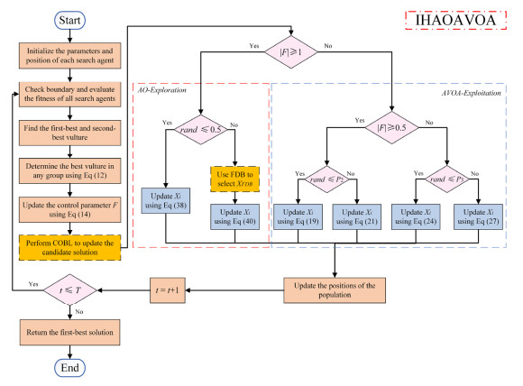
Aquila Optimizer (AO) and African Vultures Optimization Algorithm (AVOA) are two newly developed meta-heuristic algorithms that simulate several intelligent hunting behaviors of Aquila and African vulture in nature, respectively. AO has powerful global exploration capability, whereas its local exploitation phase is not stable enough. On the other hand, AVOA possesses promising exploitation capability but insufficient exploration mechanisms. Based on the characteristics of both algorithms, in this paper, we propose an improved hybrid AO and AVOA optimizer called IHAOAVOA to overcome the deficiencies in the single algorithm and provide higher-quality solutions for solving global optimization problems. First, the exploration phase of AO and the exploitation phase of AVOA are combined to retain the valuable search competence of each. Then, a new composite opposition-based learning (COBL) is designed to increase the population diversity and help the hybrid algorithm escape from the local optima. In addition, to more effectively guide the search process and balance the exploration and exploitation, the fitness-distance balance (FDB) selection strategy is introduced to modify the core position update formula. The performance of the proposed IHAOAVOA is comprehensively investigated and analyzed by comparing against the basic AO, AVOA, and six state-of-the-art algorithms on 23 classical benchmark functions and the IEEE CEC2019 test suite. Experimental results demonstrate that IHAOAVOA achieves superior solution accuracy, convergence speed, and local optima avoidance than other comparison methods on most test functions. Furthermore, the practicality of IHAOAVOA is highlighted by solving five engineering design problems. Our findings reveal that the proposed technique is also highly competitive and promising when addressing real-world optimization tasks. The source code of the IHAOAVOA is publicly available at https://doi.org/10.24433/CO.2373662.v1.
Citation: Yaning Xiao, Yanling Guo, Hao Cui, Yangwei Wang, Jian Li, Yapeng Zhang. IHAOAVOA: An improved hybrid aquila optimizer and African vultures optimization algorithm for global optimization problems[J]. Mathematical Biosciences and Engineering, 2022, 19(11): 10963-11017. doi: 10.3934/mbe.2022512
Aquila Optimizer (AO) and African Vultures Optimization Algorithm (AVOA) are two newly developed meta-heuristic algorithms that simulate several intelligent hunting behaviors of Aquila and African vulture in nature, respectively. AO has powerful global exploration capability, whereas its local exploitation phase is not stable enough. On the other hand, AVOA possesses promising exploitation capability but insufficient exploration mechanisms. Based on the characteristics of both algorithms, in this paper, we propose an improved hybrid AO and AVOA optimizer called IHAOAVOA to overcome the deficiencies in the single algorithm and provide higher-quality solutions for solving global optimization problems. First, the exploration phase of AO and the exploitation phase of AVOA are combined to retain the valuable search competence of each. Then, a new composite opposition-based learning (COBL) is designed to increase the population diversity and help the hybrid algorithm escape from the local optima. In addition, to more effectively guide the search process and balance the exploration and exploitation, the fitness-distance balance (FDB) selection strategy is introduced to modify the core position update formula. The performance of the proposed IHAOAVOA is comprehensively investigated and analyzed by comparing against the basic AO, AVOA, and six state-of-the-art algorithms on 23 classical benchmark functions and the IEEE CEC2019 test suite. Experimental results demonstrate that IHAOAVOA achieves superior solution accuracy, convergence speed, and local optima avoidance than other comparison methods on most test functions. Furthermore, the practicality of IHAOAVOA is highlighted by solving five engineering design problems. Our findings reveal that the proposed technique is also highly competitive and promising when addressing real-world optimization tasks. The source code of the IHAOAVOA is publicly available at https://doi.org/10.24433/CO.2373662.v1.

| [1] |
Y. Xiao, X. Sun, Y. Guo, S. Li, Y. Zhang, Y. Wang, An improved gorilla troops optimizer based on lens opposition-based learning and adaptive β-Hill climbing for global optimization, CMES-Comput. Model. Eng. Sci., 131 (2022), 815–850. https://doi.org/10.32604/cmes.2022.019198 doi: 10.32604/cmes.2022.019198

|
| [2] |
Y. Xiao, X. Sun, Y. Guo, H. Cui, Y. Wang, J. Li, et al., An enhanced honey badger algorithm based on Lévy flight and refraction opposition-based learning for engineering design problems, J. Intell. Fuzzy Syst., (2022), 1–24. https://doi.org/10.3233/JIFS-213206 doi: 10.3233/JIFS-213206
|
| [3] |
Q. Liu, N. Li, H. Jia, Q. Qi, L. Abualigah, Y. Liu, A hybrid arithmetic optimization and golden sine algorithm for solving industrial engineering design problems, Mathematics, 10 (2022), 1567. https://doi.org/10.3390/math10091567 doi: 10.3390/math10091567
|
| [4] |
A. S. Sadiq, A. A. Dehkordi, S. Mirjalili, Q. V. Pham, Nonlinear marine predator algorithm: a cost-effective optimizer for fair power allocation in NOMA-VLC-B5G networks, Expert Syst. Appl., 203 (2022), 117395. https://doi.org/10.1016/j.eswa.2022.117395 doi: 10.1016/j.eswa.2022.117395
|
| [5] |
G. Hu, J. Zhong, B. Du, G. Wei, An enhanced hybrid arithmetic optimization algorithm for engineering applications, Comput. Methods Appl. Mech. Eng., 394 (2022), 114901. https://doi.org/10.1016/j.cma.2022.114901 doi: 10.1016/j.cma.2022.114901
|
| [6] |
A. A. Dehkordi, A. S. Sadiq, S. Mirjalili, K. Z. Ghafoor, Nonlinear-based Chaotic harris hawks optimizer: algorithm and internet of vehicles application, Appl. Soft Comput., 109 (2021), 107574. https://doi.org/10.1016/j.asoc.2021.107574 doi: 10.1016/j.asoc.2021.107574
|
| [7] |
W. Zhao, L. Wang, S. Mirjalili, Artificial hummingbird algorithm: a new bio-inspired optimizer with its engineering applications, Comput. Methods Appl. Mech. Eng., 388 (2022), 114194. https://doi.org/10.1016/j.cma.2021.114194 doi: 10.1016/j.cma.2021.114194
|
| [8] |
K. Sun, H. Jia, Y. Li, Z. Jiang, Hybrid improved slime mould algorithm with adaptive β hill climbing for numerical optimization, J. Intell. Fuzzy Syst., 40 (2021), 1667–1679. https://doi.org/10.3233/jifs-201755 doi: 10.3233/JIFS-201755
|
| [9] |
K. Zhong, G. Zhou, W. Deng, Y. Zhou, Q. Luo, MOMPA: multi-objective marine predator algorithm, Comput. Methods Appl. Mech. Eng., 385 (2021), 114029. https://doi.org/10.1016/j.cma.2021.114029 doi: 10.1016/j.cma.2021.114029
|
| [10] |
Q. Fan, H. Huang, K. Yang, S. Zhang, L. Yao, Q. Xiong, A modified equilibrium optimizer using opposition-based learning and novel update rules, Expert Syst. Appl., 170 (2021), 114575. https://doi.org/10.1016/j.eswa.2021.114575 doi: 10.1016/j.eswa.2021.114575
|
| [11] |
L. Abualigah, A. Diabat, M. A. Elaziz, Improved slime mould algorithm by opposition-based learning and Levy flight distribution for global optimization and advances in real-world engineering problems, J. Ambient Intell. Humanized Comput., (2021), https://doi.org/10.1007/s12652-021-03372-w doi: 10.1007/s12652-021-03372-w
|
| [12] |
S. Wang, H. Jia, L. Abualigah, Q. Liu, R. Zheng, An improved hybrid aquila optimizer and harris hawks algorithm for solving industrial engineering optimization problems, Processes, 9 (2021), 1551. https://doi.org/10.3390/pr9091551 doi: 10.3390/pr9091551
|
| [13] |
L. Abualigah, A. A. Ewees, M. A. A. Al-qaness, M. A. Elaziz, D. Yousri, R. A. Ibrahim, et al., Boosting arithmetic optimization algorithm by sine cosine algorithm and levy flight distribution for solving engineering optimization problems, Neural Comput. Appl., 34 (2022), 8823–8852. https://doi.org/10.1007/s00521-022-06906-1 doi: 10.1007/s00521-022-06906-1
|
| [14] |
Y. Zhang, Y. Wang, L. Tao, Y. Yan, J. Zhao, Z. Gao, Self-adaptive classification learning hybrid JAYA and Rao-1 algorithm for large-scale numerical and engineering problems, Eng. Appl. Artif. Intell., 114 (2022), 105069. https://doi.org/10.1016/j.engappai.2022.105069 doi: 10.1016/j.engappai.2022.105069
|
| [15] |
D. Wu, H. Jia, L. Abualigah, Z. Xing, R. Zheng, H. Wang, et al., Enhance teaching-learning-based optimization for tsallis-entropy-based feature selection classification approach, Processes, 10 (2022), 360. https://doi.org/10.3390/pr10020360 doi: 10.3390/pr10020360
|
| [16] |
H. Jia, W. Zhang, R. Zheng, S. Wang, X. Leng, N. Cao, Ensemble mutation slime mould algorithm with restart mechanism for feature selection, Int. J. Intell. Syst., 37 (2021), 2335–2370. https://doi.org/10.1002/int.22776 doi: 10.1002/int.22776
|
| [17] |
H. Jia, K. Sun, Improved barnacles mating optimizer algorithm for feature selection and support vector machine optimization, Pattern Anal. Appl., 24 (2021), 1249–1274. https://doi.org/10.1007/s10044-021-00985-x doi: 10.1007/s10044-021-00985-x
|
| [18] |
C. Kumar, T. D. Raj, M. Premkumar, T. D. Raj, A new stochastic slime mould optimization algorithm for the estimation of solar photovoltaic cell parameters, Optik, 223 (2020), 165277. https://doi.org/10.1016/j.ijleo.2020.165277 doi: 10.1016/j.ijleo.2020.165277
|
| [19] |
Y. Zhang, Y. Wang, S. Li, F. Yao, L. Tao, Y. Yan, et al., An enhanced adaptive comprehensive learning hybrid algorithm of Rao-1 and JAYA algorithm for parameter extraction of photovoltaic models, Math. Biosci. Eng., 19 (2022), 5610–5637. https://doi.org/10.3934/mbe.2022263 doi: 10.3934/mbe.2022263
|
| [20] |
M. Eslami, E. Akbari, S. T. Seyed Sadr, B. F. Ibrahim, A novel hybrid algorithm based on rat swarm optimization and pattern search for parameter extraction of solar photovoltaic models, Energy Sci. Eng., (2022). https://doi.org/10.1002/ese3.1160 doi: 10.1002/ese3.1160
|
| [21] |
J. Zhao, Y. Zhang, S. Li, Y. Wang, Y. Yan, Z. Gao, A chaotic self-adaptive JAYA algorithm for parameter extraction of photovoltaic models, Math. Biosci. Eng., 19 (2022), 5638–5670. https://doi.org/10.3934/mbe.2022264 doi: 10.3934/mbe.2022264
|
| [22] |
X. Bao, H. Jia, C. Lang, A novel hybrid harris hawks optimization for color image multilevel thresholding segmentation, IEEE Access, 7 (2019), 76529–76546. https://doi.org/10.1109/access.2019.2921545 doi: 10.1109/ACCESS.2019.2921545
|
| [23] |
S. Lin, H. Jia, L. Abualigah, M. Altalhi, Enhanced slime mould algorithm for multilevel thresholding image segmentation using entropy measures, Entropy, 23 (2021), 1700. https://doi.org/10.3390/e23121700 doi: 10.3390/e23121700
|
| [24] |
M. Abd Elaziz, D. Mohammadi, D. Oliva, K. Salimifard, Quantum marine predators algorithm for addressing multilevel image segmentation, Appl. Soft Comput., 110 (2021), 107598. https://doi.org/10.1016/j.asoc.2021.107598 doi: 10.1016/j.asoc.2021.107598
|
| [25] |
J. Yao, Y. Sha, Y. Chen, G. Zhang, X. Hu, G. Bai, et al., IHSSAO: An improved hybrid salp swarm algorithm and aquila optimizer for UAV path planning in complex terrain, Appl. Sci., 12 (2022), 5634. https://doi.org/10.3390/app12115634 doi: 10.3390/app12115634
|
| [26] |
J. H. Holland, Genetic algorithms, Sci. Am., 267 (1992), 66–72. https://doi.org/10.1038/scientificamerican0792-66 doi: 10.1038/scientificamerican0792-66
|
| [27] |
P. J. Angeline, Genetic programming: On the programming of computers by means of natural selection, Biosystems, 33 (1994), 69–73. https://doi.org/10.1016/0303-2647(94)90062-0 doi: 10.1016/0303-2647(94)90062-0
|
| [28] |
R. Storn, K. Price, Differential evolution - a simple and efficient heuristic for global optimization over continuous spaces, J. Global Optim., 11 (1997), 341–359. https://doi.org/10.1023/A:1008202821328 doi: 10.1023/A:1008202821328
|
| [29] |
H. G. Beyer, H. P. Schwefel, Evolution strategies-A comprehensive introduction, Nat. Comput., 1 (2002), 3–52. https://doi.org/10.1023/A:1015059928466 doi: 10.1023/A:1015059928466
|
| [30] |
D. Simon, Biogeography-based optimization, IEEE Trans. Evol. Comput., 12 (2008), 702–713. https://doi.org/10.1109/TEVC.2008.919004 doi: 10.1109/TEVC.2008.919004
|
| [31] |
S. Kirkpatrick, C. D. Gelatt, M. P. Vecchi, Optimization by simulated annealing, Science, 220 (1983), 671–680. https://doi.org/10.1126/science.220.4598.671 doi: 10.1126/science.220.4598.671
|
| [32] |
E. Rashedi, H. Nezamabadi-pour, S. Saryazdi, GSA: a gravitational search algorithm, Inf. Sci., 179 (2009), 2232–2248. https://doi.org/10.1016/j.ins.2009.03.004 doi: 10.1016/j.ins.2009.03.004
|
| [33] |
S. Mirjalili, S. M. Mirjalili, A. Hatamlou, Multi-Verse Optimizer: a nature-inspired algorithm for global optimization, Neural Comput. Appl., 27 (2016), 495–513. https://doi.org/10.1007/s00521-015-1870-7 doi: 10.1007/s00521-015-1870-7
|
| [34] |
W. Zhao, L. Wang, Z. Zhang, Atom search optimization and its application to solve a hydrogeologic parameter estimation problem, Knowl.-Based Syst., 163 (2019), 283–304. https://doi.org/10.1016/j.knosys.2018.08.030 doi: 10.1016/j.knosys.2018.08.030
|
| [35] |
A. Hatamlou, Black hole: a new heuristic optimization approach for data clustering, Inf. Sci., 222 (2013), 175–184. https://doi.org/10.1016/j.ins.2012.08.023 doi: 10.1016/j.ins.2012.08.023
|
| [36] |
S. Mirjalili, SCA: a sine cosine algorithm for solving optimization problems, Knowl.-Based Syst., 96 (2016), 120–133. https://doi.org/10.1016/j.knosys.2015.12.022 doi: 10.1016/j.knosys.2015.12.022
|
| [37] |
A. Kaveh, A. Dadras, A novel meta-heuristic optimization algorithm: thermal exchange optimization, Adv. Eng. Software, 110 (2017), 69–84. https://doi.org/10.1016/j.advengsoft.2017.03.014 doi: 10.1016/j.advengsoft.2017.03.014
|
| [38] |
L. Abualigah, A. Diabat, S. Mirjalili, M. Abd Elaziz, A. H. Gandomi, The arithmetic optimization algorithm, Comput. Methods Appl. Mech. Eng., 376 (2021), 113609. https://doi.org/10.1016/j.cma.2020.113609 doi: 10.1016/j.cma.2020.113609
|
| [39] | J. Kennedy, R. Eberhart, Particle swarm optimization, in Proceedings of ICNN'95 - International Conference on Neural Networks, (1995), 1942–1948. https://doi.org/10.1109/ICNN.1995.488968 |
| [40] |
M. Dorigo, M. Birattari, T. Stutzle, Ant colony optimization, IEEE Comput. Intell. Mag., 1 (2006), 28–39. https://doi.org/10.1109/MCI.2006.329691 doi: 10.1109/MCI.2006.329691
|
| [41] |
S. Mirjalili, Dragonfly algorithm: a new meta-heuristic optimization technique for solving single-objective, discrete, and multi-objective problems, Neural Comput. Appl., 27 (2015), 1053–1073. https://doi.org/10.1007/s00521-015-1920-1 doi: 10.1007/s00521-015-1920-1
|
| [42] |
S. Mirjalili, The ant lion optimizer, Adv. Eng. Software, 83 (2015), 80–98. https://doi.org/10.1016/j.advengsoft.2015.01.010 doi: 10.1016/j.advengsoft.2015.01.010
|
| [43] |
S. Mirjalili, A. Lewis, The whale optimization algorithm, Adv. Eng. Software, 95 (2016), 51–67. https://doi.org/10.1016/j.advengsoft.2016.01.008 doi: 10.1016/j.advengsoft.2016.01.008
|
| [44] |
S. Mirjalili, S. M. Mirjalili, A. Lewis, Grey wolf optimizer, Adv. Eng. Software, 69 (2014), 46–61. https://doi.org/10.1016/j.advengsoft.2013.12.007 doi: 10.1016/j.advengsoft.2013.12.007
|
| [45] |
S. Mirjalili, A. H. Gandomi, S. Z. Mirjalili, S. Saremi, H. Faris, S. M. Mirjalili, Salp swarm algorithm: a bio-inspired optimizer for engineering design problems, Adv. Eng. Software, 114 (2017), 163–191. https://doi.org/10.1016/j.advengsoft.2017.07.002 doi: 10.1016/j.advengsoft.2017.07.002
|
| [46] |
F. Glover, Tabu search—Part Ⅰ, ORSA J. Comput., 1 (1989), 190–206. https://doi.org/10.1287/ijoc.1.3.190 doi: 10.1287/ijoc.1.3.190
|
| [47] |
D. Manjarres, I. Landa-Torres, S. Gil-Lopez, J. Del Ser, M. N. Bilbao, S. Salcedo-Sanz, et al., A survey on applications of the harmony search algorithm, Eng. Appl. Artif. Intell., 26 (2013), 1818–1831. https://doi.org/10.1016/j.engappai.2013.05.008 doi: 10.1016/j.engappai.2013.05.008
|
| [48] |
M. S. Gonçalves, R. H. Lopez, L. F. F. Miguel, Search group algorithm: a new metaheuristic method for the optimization of truss structures, Comput. Struct., 153 (2015), 165–184. https://doi.org/10.1016/j.compstruc.2015.03.003 doi: 10.1016/j.compstruc.2015.03.003
|
| [49] |
E. Atashpaz-Gargari, C. Lucas, Imperialist competitive algorithm: an algorithm for optimization inspired by imperialistic competition, 2007 IEEE Congr. Evol. Comput., (2007), 4661–4667. https://doi.org/10.1109/CEC.2007.4425083 doi: 10.1109/CEC.2007.4425083
|
| [50] |
R. V. Rao, V. J. Savsani, D. P. Vakharia, Teaching–learning-based optimization: a novel method for constrained mechanical design optimization problems, Comput.Aided Des., 43 (2011), 303–315. https://doi.org/10.1016/j.cad.2010.12.015 doi: 10.1016/j.cad.2010.12.015
|
| [51] |
S. Mirjalili, Moth-flame optimization algorithm: a novel nature-inspired heuristic paradigm, Knowl.-Based Syst., 89 (2015), 228–249. https://doi.org/10.1016/j.knosys.2015.07.006 doi: 10.1016/j.knosys.2015.07.006
|
| [52] |
S. Li, H. Chen, M. Wang, A. A. Heidari, S. Mirjalili, Slime mould algorithm: a new method for stochastic optimization, Future Gener. Comput. Syst., 111 (2020), 300–323. https://doi.org/10.1016/j.future.2020.03.055 doi: 10.1016/j.future.2020.03.055
|
| [53] |
S. Kaur, L. K. Awasthi, A. L. Sangal, G. Dhiman, Tunicate swarm algorithm: a new bio-inspired based metaheuristic paradigm for global optimization, Eng. Appl. Artif. Intell., 90 (2020), 103541. https://doi.org/10.1016/j.engappai.2020.103541 doi: 10.1016/j.engappai.2020.103541
|
| [54] |
A. A. Heidari, S. Mirjalili, H. Faris, I. Aljarah, M. Mafarja, H. Chen, Harris hawks optimization: algorithm and applications, Future Gener. Comput. Syst., 97 (2019), 849–872. https://doi.org/10.1016/j.future.2019.02.028 doi: 10.1016/j.future.2019.02.028
|
| [55] |
B. Abdollahzadeh, F. Soleimanian Gharehchopogh, S. Mirjalili, Artificial gorilla troops optimizer: a new nature‐inspired metaheuristic algorithm for global optimization problems, Int. J. Intell. Syst., 36 (2021), 5887–5958. https://doi.org/10.1002/int.22535 doi: 10.1002/int.22535
|
| [56] |
H. Jia, X. Peng, C. Lang, Remora optimization algorithm, Expert Syst. Appl., 185 (2021), 115665. https://doi.org/10.1016/j.eswa.2021.115665 doi: 10.1016/j.eswa.2021.115665
|
| [57] |
Y. Yang, H. Chen, A. A. Heidari, A. H. Gandomi, Hunger games search: visions, conception, implementation, deep analysis, perspectives, and towards performance shifts, Expert Syst. Appl., 177 (2021), 114864. https://doi.org/10.1016/j.eswa.2021.114864 doi: 10.1016/j.eswa.2021.114864
|
| [58] |
L. Abualigah, M. A. Elaziz, P. Sumari, Z. W. Geem, A. H. Gandomi, Reptile search algorithm (RSA): a nature-inspired meta-heuristic optimizer, Expert Syst. Appl., 191 (2022), 116158. https://doi.org/10.1016/j.eswa.2021.116158 doi: 10.1016/j.eswa.2021.116158
|
| [59] |
Y. Xiao, X. Sun, Y. Zhang, Y. Guo, Y. Wang, J. Li, An improved slime mould algorithm based on Tent chaotic mapping and nonlinear inertia weight, Int. J. Innovative Comput. Inf. Control, 17 (2021), 2151–2176. https://doi.org/10.24507/ijicic.17.06.2151 doi: 10.24507/ijicic.17.06.2151
|
| [60] |
R. Zheng, H. Jia, L. Abualigah, Q. Liu, S. Wang, Deep ensemble of slime mold algorithm and arithmetic optimization algorithm for global optimization, Processes, 9 (2021), 1774. https://doi.org/10.3390/pr9101774 doi: 10.3390/pr9101774
|
| [61] |
H. Jia, K. Sun, W. Zhang, X. Leng, An enhanced chimp optimization algorithm for continuous optimization domains, Complex Intell. Syst., 8 (2022), 65–82. https://doi.org/10.1007/s40747-021-00346-5 doi: 10.1007/s40747-021-00346-5
|
| [62] |
A. S. Sadiq, A. A. Dehkordi, S. Mirjalili, J. Too, P. Pillai, Trustworthy and efficient routing algorithm for IoT-FinTech applications using non-linear Lévy brownian generalized normal distribution optimization, IEEE Internet Things J., (2021), 1–16. https://doi.org/10.1109/jiot.2021.3109075 doi: 10.1109/jiot.2021.3109075
|
| [63] |
D. H. Wolpert, W. G. Macready, No free lunch theorems for optimization, IEEE Trans. Evol. Comput., 1 (1997), 67–82. https://doi.org/10.1109/4235.585893 doi: 10.1109/4235.585893
|
| [64] |
S. Chakraborty, A. K. Saha, R. Chakraborty, M. Saha, S. Nama, HSWOA: an ensemble of hunger games search and whale optimization algorithm for global optimization, Int. J. Intell. Syst., 37 (2022), 52–104. https://doi.org/10.1002/int.22617 doi: 10.1002/int.22617
|
| [65] |
P. Pirozmand, A. Javadpour, H. Nazarian, P. Pinto, S. Mirkamali, F. Ja'fari, GSAGA: A hybrid algorithm for task scheduling in cloud infrastructure, J. Supercomput., (2022). https://doi.org/10.1007/s11227-022-04539-8 doi: 10.1007/s11227-022-04539-8
|
| [66] |
H. Abdel-Mawgoud, S. Kamel, A. A. A. El-Ela, F. Jurado, Optimal allocation of DG and capacitor in distribution networks using a novel hybrid MFO-SCA method, Electr. Power Compon. Syst., 49 (2021), 259–275. https://doi.org/10.1080/15325008.2021.1943066 doi: 10.1080/15325008.2021.1943066
|
| [67] |
L. Abualigah, D. Yousri, M. Abd Elaziz, A. A. Ewees, M. A. A. Al-qaness, A. H. Gandomi, Aquila optimizer: a novel meta-heuristic optimization algorithm, Comput. Ind. Eng., 157 (2021), 107250. https://doi.org/10.1016/j.cie.2021.107250 doi: 10.1016/j.cie.2021.107250
|
| [68] |
B. Abdollahzadeh, F. S. Gharehchopogh, S. Mirjalili, African vultures optimization algorithm: a new nature-inspired metaheuristic algorithm for global optimization problems, Comput. Ind. Eng., 158 (2021), 107408. https://doi.org/10.1016/j.cie.2021.107408 doi: 10.1016/j.cie.2021.107408
|
| [69] |
Z. Guo, B. Yang, Y. Han, T. He, P. He, X. Meng, et al., Optimal PID tuning of PLL for PV inverter based on aquila optimizer, Front. Energy Res., 9 (2022), 812467. https://doi.org/10.3389/fenrg.2021.812467 doi: 10.3389/fenrg.2021.812467
|
| [70] |
M. R. Hussan, M. I. Sarwar, A. Sarwar, M. Tariq, S. Ahmad, A. Shah Noor Mohamed, et al., Aquila optimization based harmonic elimination in a modified H-bridge inverter, Sustainability, 14 (2022), 929. https://doi.org/10.3390/su14020929 doi: 10.3390/su14020929
|
| [71] |
G. Vashishtha, R. Kumar, Autocorrelation energy and aquila optimizer for MED filtering of sound signal to detect bearing defect in Francis turbine, Meas. Sci. Technol., 33 (2021), 015006. https://doi.org/10.1088/1361-6501/ac2cf2 doi: 10.1088/1361-6501/ac2cf2
|
| [72] |
A. M. AlRassas, M. A. A. Al-qaness, A. A. Ewees, S. Ren, M. Abd Elaziz, R. Damaševičius, et al., Optimized ANFIS model using Aquila optimizer for oil production forecasting, Processes, 9 (2021), 1194. https://doi.org/10.3390/pr9071194 doi: 10.3390/pr9071194
|
| [73] |
A. K. Khamees, A. Y. Abdelaziz, M. R. Eskaros, A. El-Shahat, M. A. Attia, Optimal power flow solution of wind-integrated power system using novel metaheuristic method, Energies, 14 (2021), 6117. https://doi.org/10.3390/en14196117 doi: 10.3390/en14196117
|
| [74] |
J. Zhao, Z. M. Gao, The heterogeneous Aquila optimization algorithm, Math. Biosci. Eng., 19 (2022), 5867–5904. https://doi.org/10.3934/mbe.2022275 doi: 10.3934/mbe.2022275
|
| [75] |
M. Kandan, A. Krishnamurthy, S. A. M. Selvi, M. Y. Sikkandar, M. A. Aboamer, T. Tamilvizhi, Quasi oppositional Aquila optimizer-based task scheduling approach in an IoT enabled cloud environment, J. Supercomput., 78 (2022), 10176–10190. https://doi.org/10.1007/s11227-022-04311-y doi: 10.1007/s11227-022-04311-y
|
| [76] |
X. Li, S. Mobayen, Optimal design of a PEMFC‐based combined cooling, heating and power system based on an improved version of Aquila optimizer, Concurrency Comput. Pract. Exper., 34 (2022), e6976. https://doi.org/10.1002/cpe.6976 doi: 10.1002/cpe.6976
|
| [77] |
J. Zhao, Z. M. Gao, H. F. Chen, The simplified aquila optimization algorithm, IEEE Access, 10 (2022), 22487–22515. https://doi.org/10.1109/access.2022.3153727 doi: 10.1109/ACCESS.2022.3153727
|
| [78] |
S. Mahajan, L. Abualigah, A. K. Pandit, M. Altalhi, Hybrid Aquila optimizer with arithmetic optimization algorithm for global optimization tasks, Soft Comput., 26 (2022), 4863–4881. https://doi.org/10.1007/s00500-022-06873-8 doi: 10.1007/s00500-022-06873-8
|
| [79] |
Y. Zhang, Y. Yan, J. Zhao, Z. Gao, AOAAO: The hybrid algorithm of arithmetic optimization algorithm with aquila optimizer, IEEE Access, 10 (2022), 10907–10933. https://doi.org/10.1109/access.2022.3144431 doi: 10.1109/ACCESS.2022.3144431
|
| [80] |
G. Vashishtha, S. Chauhan, A. Kumar, R. Kumar, An ameliorated African vulture optimization algorithm to diagnose the rolling bearing defects, Meas. Sci. Technol., 33 (2022), 075013. https://doi.org/10.1088/1361-6501/ac656a doi: 10.1088/1361-6501/ac656a
|
| [81] |
M. R. Kaloop, B. Roy, K. Chaurasia, S. M. Kim, H. M. Jang, J. W. Hu, et al., Shear strength estimation of reinforced concrete deep beams using a novel hybrid metaheuristic optimized SVR models, Sustainability, 14 (2022), 5238. https://doi.org/10.3390/su14095238 doi: 10.3390/su14095238
|
| [82] |
M. Manickam, R. Siva, S. Prabakeran, K. Geetha, V. Indumathi, T. Sethukarasi, Pulmonary disease diagnosis using African vulture optimized weighted support vector machine approach, Int. J. Imaging Syst. Technol., 32 (2022), 843–856. https://doi.org/https://doi.org/10.1002/ima.22669 doi: 10.1002/ima.22669
|
| [83] |
J. Fan, Y. Li, T. Wang, An improved African vultures optimization algorithm based on tent chaotic mapping and time-varying mechanism, PLoS One, 16 (2021), e0260725. https://doi.org/10.1371/journal.pone.0260725 doi: 10.1371/journal.pone.0260725
|
| [84] | H. R. Tizhoosh, Opposition-based learning: a new scheme for machine intelligence, in International Conference on Computational Intelligence for Modelling, Control and Automation and International Conference on Intelligent Agents, Web Technologies and Internet Commerce, (2005), 695–701. https://doi.org/10.1109/CIMCA.2005.1631345 |
| [85] |
N. A. Alawad, B. H. Abed-alguni, Discrete island-based cuckoo search with highly disruptive polynomial mutation and opposition-based learning strategy for scheduling of workflow applications in cloud environments, Arabian J. Sci. Eng., 46 (2021), 3213–3233. https://doi.org/10.1007/s13369-020-05141-x doi: 10.1007/s13369-020-05141-x
|
| [86] |
T. T. Nguyen, H. J. Wang, T. K. Dao, J. S. Pan, J. H. Liu, S. Weng, An improved slime mold algorithm and its application for optimal operation of cascade hydropower stations, IEEE Access, 8 (2020), 226754–226772. https://doi.org/10.1109/access.2020.3045975 doi: 10.1109/access.2020.3045975
|
| [87] |
Y. Zhang, Y. Wang, Y. Yan, J. Zhao, Z. Gao, LMRAOA: an improved arithmetic optimization algorithm with multi-leader and high-speed jumping based on opposition-based learning solving engineering and numerical problems, Alexandria Eng. J., 61 (2022), 12367–12403. https://doi.org/10.1016/j.aej.2022.06.017 doi: 10.1016/j.aej.2022.06.017
|
| [88] |
S. Wang, H. Jia, Q. Liu, R. Zheng, An improved hybrid Aquila optimizer and Harris Hawks optimization for global optimization, Math. Biosci. Eng., 18 (2021), 7076–7109. https://doi.org/10.3934/mbe.2021352 doi: 10.3934/mbe.2021352
|
| [89] |
Q. Fan, Z. Chen, W. Zhang, X. Fang, ESSAWOA: Enhanced whale optimization algorithm integrated with salp swarm algorithm for global optimization, Eng. Comput., 38 (2022), 797–814. https://doi.org/10.1007/s00366-020-01189-3 doi: 10.1007/s00366-020-01189-3
|
| [90] |
F. Yu, Y. Li, B. Wei, X. Xu, Z. Zhao, The application of a novel OBL based on lens imaging principle in PSO, Acta Electron. Sin., 42 (2014), 230–235. https://doi.org/10.3969/j.issn.0372-2112.2014.02.004 doi: 10.3969/j.issn.0372-2112.2014.02.004
|
| [91] |
W. Long, J. Jiao, X. Liang, S. Cai, M. Xu, A random opposition-based learning grey wolf optimizer, IEEE Access, 7 (2019), 113810–113825. https://doi.org/10.1109/access.2019.2934994 doi: 10.1109/access.2019.2934994
|
| [92] |
H. T. Kahraman, H. Bakir, S. Duman, M. Katı, S. Aras, U. Guvenc, Dynamic FDB selection method and its application: modeling and optimizing of directional overcurrent relays coordination, Appl. Intell., 52 (2022), 4873–4908. https://doi.org/10.1007/s10489-021-02629-3 doi: 10.1007/s10489-021-02629-3
|
| [93] |
H. T. Kahraman, S. Aras, E. Gedikli, Fitness-distance balance (FDB): a new selection method for meta-heuristic search algorithms, Knowl.-Based Syst., 190 (2020), 105169. https://doi.org/10.1016/j.knosys.2019.105169 doi: 10.1016/j.knosys.2019.105169
|
| [94] |
S. Aras, E. Gedikli, H. T. Kahraman, A novel stochastic fractal search algorithm with fitness-distance balance for global numerical optimization, Swarm Evol. Comput., 61 (2021), 100821. https://doi.org/10.1016/j.swevo.2020.100821 doi: 10.1016/j.swevo.2020.100821
|
| [95] |
S. Duman, H. T. Kahraman, U. Guvenc, S. Aras, Development of a Lévy flight and FDB-based coyote optimization algorithm for global optimization and real-world ACOPF problems, Soft Comput., 25 (2021), 6577–6617. https://doi.org/10.1007/s00500-021-05654-z doi: 10.1007/s00500-021-05654-z
|
| [96] |
S. García, A. Fernández, J. Luengo, F. Herrera, Advanced nonparametric tests for multiple comparisons in the design of experiments in computational intelligence and data mining: Experimental analysis of power, Inf. Sci., 180 (2010), 2044–2064. https://doi.org/10.1016/j.ins.2009.12.010 doi: 10.1016/j.ins.2009.12.010
|
| [97] |
E. Theodorsson-Norheim, Friedman and Quade tests: basic computer program to perform nonparametric two-way analysis of variance and multiple comparisons on ranks of several related samples, Comput. Biol. Med., 17 (1987), 85–99. https://doi.org/10.1016/0010-4825(87)90003-5 doi: 10.1016/0010-4825(87)90003-5
|
| [98] | K. V. Price, N. H. Awad, M. Z. Ali, P. N. Suganthan, The 100-digit challenge: problem definitions and evaluation criteria for the 100-digit challenge special session and competition on single objective numerical optimization. Technical Report Nanyang Technological University, Singapore, (2018). |
| [99] |
C. A. Coello Coello, Theoretical and numerical constraint-handling techniques used with evolutionary algorithms: a survey of the state of the art, Comput. Methods Appl. Mech. Eng., 191 (2002), 1245–1287. https://doi.org/10.1016/S0045-7825(01)00323-1 doi: 10.1016/S0045-7825(01)00323-1
|
Figures(15) / Tables(17)

Yaning Xiao, Yanling Guo, Hao Cui, Yangwei Wang, Jian Li, Yapeng Zhang. IHAOAVOA: An improved hybrid aquila optimizer and African vultures optimization algorithm for global optimization problems[J]. Mathematical Biosciences and Engineering, 2022, 19(11): 10963-11017. doi: 10.3934/mbe.2022512


 DownLoad: