Model and application of farmers' credit risk early warning system based on T-S fuzzy neural network application

Hui Wang; Hui Wang

doi:10.3934/mbe.2022368

Mathematical Biosciences and Engineering

2022, Volume 19, Issue 8: 7886-7898. doi: 10.3934/mbe.2022368

Previous Article Next Article

Research article Special Issues

Model and application of farmers' credit risk early warning system based on T-S fuzzy neural network application

Hui Wang ^,

College of Economics, Northwest University of Political Science and Law, Shaanxi, 710000, China

Received: 07 April 2022 Revised: 29 April 2022 Accepted: 17 May 2022 Published: 27 May 2022

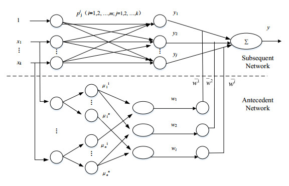
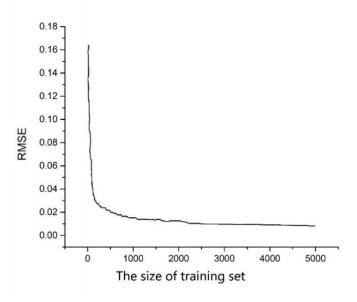
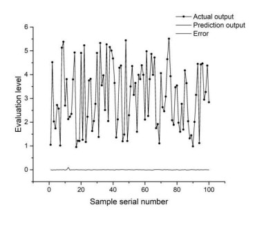
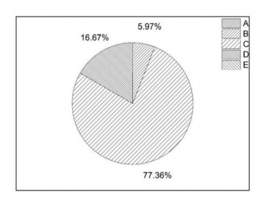
In China, farmers' loan difficulties have become a major problem restricting increases in farmers' incomes and the economic development of rural areas. The existing studies of the management and control of farmers' credit risk have mostly been pre-management, which cannot efficiently prevent and reduce the occurrence of farmers' credit risk in time. This paper uses the T-S neural network model to build a farmers' credit risk early warning system so that formal financial institutions can predict the occurrence of and changes in the farmers' credit risks in a timely manner and quickly undertake countermeasures to reduce losses. After training and testing, a model with a higher degree of fit is used to analyze the credit level of farmers in Shaanxi Province from 2016 to 2018. The results demonstrate that the credit level of farmers in this area is continuously improving, in agreement with the actual situation. The results also show that the prediction accuracy of the T-S fuzzy neural network is high, verifying the rationality of the selection of test samples.

Keywords:

Citation: Hui Wang. Model and application of farmers' credit risk early warning system based on T-S fuzzy neural network application[J]. Mathematical Biosciences and Engineering, 2022, 19(8): 7886-7898. doi: 10.3934/mbe.2022368

Related Papers:

[1]	Jehad Shaikhali, Gunnar Wingsle . Redox-regulated transcription in plants: Emerging concepts. AIMS Molecular Science, 2017, 4(3): 301-338. doi: 10.3934/molsci.2017.3.301
[2]	Amedea B. Seabra, Halley C. Oliveira . How nitric oxide donors can protect plants in a changing environment: what we know so far and perspectives. AIMS Molecular Science, 2016, 3(4): 692-718. doi: 10.3934/molsci.2016.4.692
[3]	Vittorio Emanuele Bianchi, Giancarlo Falcioni . Reactive oxygen species, health and longevity. AIMS Molecular Science, 2016, 3(4): 479-504. doi: 10.3934/molsci.2016.4.479
[4]	Luís J. del Valle, Lourdes Franco, Ramaz Katsarava, Jordi Puiggalí . Electrospun biodegradable polymers loaded with bactericide agents. AIMS Molecular Science, 2016, 3(1): 52-87. doi: 10.3934/molsci.2016.1.52
[5]	Isabella Martins Lourenço, Amedea Barozzi Seabra, Marcelo Lizama Vera, Nicolás Hoffmann, Olga Rubilar Araneda, Leonardo Bardehle Parra . Synthesis and application of zinc oxide nanoparticles in Pieris brassicae larvae as a possible pesticide effect. AIMS Molecular Science, 2024, 11(4): 351-366. doi: 10.3934/molsci.2024021
[6]	Vahid Pouresmaeil, Marwa Mawlood Salman Al-zand, Aida Pouresmaeil, Seyedeh Samira Saghravanian, Masoud Homayouni Tabrizi . Loading diltiazem onto surface-modified nanostructured lipid carriers to evaluate its apoptotic, cytotoxic, and inflammatory effects on human breast cancer cells. AIMS Molecular Science, 2024, 11(3): 231-250. doi: 10.3934/molsci.2024014
[7]	Giulia Ambrosi, Pamela Milani . Endoplasmic reticulum, oxidative stress and their complex crosstalk in neurodegeneration: proteostasis, signaling pathways and molecular chaperones. AIMS Molecular Science, 2017, 4(4): 424-444. doi: 10.3934/molsci.2017.4.424
[8]	Davide Lovisolo, Marianna Dionisi, Federico A. Ruffinatti, Carla Distasi . Nanoparticles and potential neurotoxicity: focus on molecular mechanisms. AIMS Molecular Science, 2018, 5(1): 1-13. doi: 10.3934/molsci.2018.1.1
[9]	Zhaoping Qin, Patrick Robichaud, Taihao Quan . Oxidative stress and CCN1 protein in human skin connective tissue aging. AIMS Molecular Science, 2016, 3(2): 269-279. doi: 10.3934/molsci.2016.2.269
[10]	Morgan Robinson, Brenda Yasie Lee, Zoya Leonenko . Drugs and drug delivery systems targeting amyloid-β in Alzheimer's disease. AIMS Molecular Science, 2015, 2(3): 332-358. doi: 10.3934/molsci.2015.3.332

Abstract

1. Introduction

Nonlinear partial differential equation is a very important branch of the nonlinear science, which has been called the foreword and hot topic of current scientific development. In theoretical science and practical application, nonlinear partial differential is used to describe the problems in the fields of optics, mechanics, communication, control science and biology ^{[1,2,3,4,5,6,7,8,9]}. At present, the main problems in the study of nonlinear partial differential equations are the existence of solutions, the stability of solutions, numerical solutions and exact solutions. With the development of research, especially the study of exact solutions of nonlinear partial differential equations has important theoretical value and application value. In the last half century, many important methods for constructing exact solutions of nonlinear partial differential equations have been proposed, such as the planar dynamic system method ^[10], the Jacobi elliptic function method ^[11], the bilinear transformation method ^[12], the complete discriminant system method for polynomials ^[13], the unified Riccati equation method ^[14], the generalized Kudryashov method ^[15], and so on ^{[16,17,18,19,20,21,22,23,24]}.

There is no unified method to obtain the exact solution of nonlinear partial differential equations. Although predecessors have obtained some analytical solutions with different methods, no scholar has studied the system with complete discrimination system for polynomial method.

The Fokas system is a very important class of nonlinear partial differential equations. In this article, we focus on the Fokas system, which is given as follows ^{[25,26,27,28,29,30,31,32,33,34,35,36,37]}

$\left\{ \begin{array}{l} i{p_t} + {r_1}{p_{xx}} + {r_2}pq = 0, \hfill \\ {r_3}{q_y} - {r_4}{(|p{|^2})_x} = 0, \hfill \end{array} \right.$

(1.1)

where $p = p(x, y, t)$ and $q = q(x, y, t)$ are the complex functions which stand for the nonlinear pulse propagation in monomode optical fibers. The parameters ${r_1}, {r_2}, {r_3}$ and ${r_4}$ are arbitrary non-zero constants, which are coefficients of nonlinear terms in Eq (1.1) and reflect different states of optical solitons.

This paper is arranged as follows. In Section 2, we describe the method of the complete discrimination system for polynomial method. In Section 3, we substitute traveling wave transformation into nonlinear ordinary differential equations and obtain the different new single traveling wave solutions for the Fokas system by complete discrimination system for polynomial method. At the same time, we draw some images of solutions. In Section 4, the main results are summarized.

2. Description of the method

First, we consider the following partial differential equations:

$\left\{ \begin{array}{l}F(u, v, {u}_{x}, {u}_{t}, {v}_{x}, {v}_{t}, {u}_{xx}, {u}_{xt}, {u}_{tt}, \cdots ) = 0\text{, }\\ G(u, v, {u}_{x}, {u}_{t}, {v}_{x}, {v}_{t}, {u}_{xx}, {u}_{xt}, {u}_{tt}, \cdots ) = 0\text{, }\end{array} \right.$

(2.1)

where $F$ and $G$ is polynomial function which is about the partial derivatives of each order of $u(x, t)$ and $v(x, t)$ with respect to $x$ and $t$ .

Step 1: Taking the traveling wave transformation $u(x, t) = u(\xi), v(x, t) = v(\xi), \xi = kx + ct$ into Eq (2.1), then the partial differential equation is converted to an ordinary differential equation

$\left\{ \begin{array}{l} F(u, v, u', v', u'', v'', \cdots ) = 0, \hfill \\ G(u, v, u', v', u'', v'', \cdots ) = 0. \hfill \end{array} \right.$

(2.2)

Step 2: The above nonlinear ordinary differential equations (2.2) are reduced to the following ordinary differential form after a series of transformations:

${(u')^2} = {u^3} + {d_2}{u^2} + {d_1}u + {d_0}.$

(2.3)

The Eq (2.3) can also be written in integral form as:

$\pm (\xi - {\xi _0}) = \int {\frac{{du}}{{\sqrt {{u^3} + {d_2}{u^2} + {d_1}u + {d_0}} }}} .$

(2.4)

Step 3: Let $\phi (u) = {u^3} + {d_2}{u^2} + {d_1}u + {d_0}$ . According to the complete discriminant system method of third-order polynomial

$\left\{\begin{array}{l} \Delta=-27(\frac{2 d_2^3}{27}+d_0-\frac{d_1 d_2}{3})^2-4(d_1-\frac{d_2^2}{3})^3, \\ D_1=d_1-\frac{d_2^2}{3}, \end{array}\right.$

(2.5)

the classification of the solution of the equation can be obtained, and the classification of traveling wave solution of the Fokas system will be given in the following section.

3. Traveling wave solution of Eq (1.1)

In the current part, we obtain all exact solutions to Eq (1.1) by complete discrimination system for polynomial method. According to the wave transformation

$p(x, y, t) = \varphi (\eta ){e^{i({\lambda _1}x + {\lambda _2}y + {\lambda _3}t + {\lambda _4})}}, q(x, y, t) = \phi (\eta ), \eta = x + y - vt,$

(3.1)

where ${\lambda _1}, {\lambda _2}, {\lambda _3}, {\lambda _4}$ and $v$ are real parameters, and $v$ represents the wave frame speed.

Substituting the above transformation Eq (3.1) into Eq (1.1), we get

$\left\{ \begin{array}{l} ( - v + 2{r_1}{\lambda _1})i\varphi ' - {\lambda _3}\varphi + {r_1}\varphi '' - {r_1}\lambda _1^2\varphi + {r_2}\varphi \phi = 0, \hfill \\ {r_3}\phi ' - 2{r_4}\varphi \varphi ' = 0. \hfill \end{array} \right.$

(3.2)

Integrating the second equation in (3.2) and ignoring the integral constant, we get

$\phi (\eta ) = \frac{{{r_4}{\varphi ^2}(\eta )}}{{{r_3}}}.$

(3.3)

Substituting Eq (3.3) into the first equation in (3.2) and setting $v = 2{r_1}{\lambda _1},$ we get the following:

${r_1}\varphi '' - ({\lambda _3} + {r_1}\lambda _1^2)\varphi + \frac{{{r_2}{r_4}{\varphi ^3}}}{{{r_3}}} = 0.$

(3.4)

Multiplying $\varphi '$ both sides of the Eq (3.4), then integrating once to get

${(\varphi ')^2} = {a_4}{\varphi ^4} + {a_2}{\varphi ^2} + {a_0},$

(3.5)

where ${a_4} = - \frac{{{r_2}{r_4}}}{{2{r_1}{r_3}}}, {a_2} = \frac{{{\lambda _3} + {r_1}\lambda _1^2}}{{{r_1}}},$ ${a_0}$ is the arbitrary constant.

${\rm{Let}} \ \ \varphi = \pm \sqrt {{{(4{a_4})}^{ - \frac{1}{3}}}\omega } , \ {b_1} = 4{a_2}{(4{a_4})^{ - \frac{2}{3}}}, {b_0} = 4{a_0}{(4{a_4})^{ - \frac{1}{3}}}, {\eta _1} = {(4{a_4})^{\frac{1}{3}}}\eta .$

(3.6)

Equation (3.5) can be expressed as the following:

${({\omega '_{{\eta _1}}})^2} = {\omega ^3} + {b_1}{\omega ^2} + {b_0}\omega .$

(3.7)

Then we can get the integral expression of Eq (3.7)

$\pm ({\eta _1} - {\eta _0}) = \int {\frac{{d\omega }}{{\sqrt {\omega ({\omega ^2} + {b_1}\omega + {b_0})} }}} ,$

(3.8)

where ${\eta _0}$ is the constant of integration.

Here, we get the $F(\omega) = {\omega ^2} + {b_1}\omega + {b_0}$ and $\Delta = b_1^2 - 4{b_0}.$ In order to solve Eq (3.7), we discuss the third order polynomial discrimination system in four cases.

Case 1: $\Delta = 0$ and $\omega \gt 0.$

When ${b_1} \lt 0,$ the solution of Eq (3.7) is

${\omega _1} = - \frac{{{b_1}}}{2}{\tanh ^2}(\frac{1}{2}\sqrt { - \frac{{{b_1}}}{2}} ({\eta _1} - {\eta _0})).$

(3.9)

${\omega _2} = - \frac{{{b_1}}}{2}{\coth ^2}(\frac{1}{2}\sqrt { - \frac{{{b_1}}}{2}} ({\eta _1} - {\eta _0})).$

(3.10)

Thus, the classification of all solutions of Eq (3.7) is obtained by the third order polynomial discrimination system. The exact traveling wave solutions of the Eq (1.1) are obtained by combining the above solutions and the conditions (3.6) with Eq (3.1), can be expressed as below:

${p_1}(x, y, t) = \pm \sqrt {\frac{{{r_3}({\lambda _3} + {r_1}\lambda _1^2)}}{{{r_2}{r_4}}}} \tanh (\frac{1}{2}\sqrt { - \frac{{2({\lambda _3} + {r_1}\lambda _1^2)}}{{{r_1}}} \cdot {{(\frac{{2{r_2}{r_4}}}{{{r_1}{r_3}}})}^{^{ - \frac{2}{3}}}}} \cdot ({(\frac{{2{r_2}{r_4}}}{{{r_1}{r_3}}})^{^{\frac{1}{3}}}}\eta + {\eta _0})) \cdot {e^{i({\lambda _1}x + {\lambda _2}y + {\lambda _3}t + {\lambda _4})}}.$

(3.11)

In Eq (3.11), ${p_1}(x, y, t)$ is a dark soliton solution, it expresses the energy depression on a certain intensity background. Figure 1 depict two-dimensional graph, three-dimensional graph, contour plot and density plot of the solution.

${q_1}(x, y, t) = \frac{{{\lambda _3} + {r_1}\lambda _1^2}}{{{r_2}}}{\tanh ^2}(\frac{1}{2}\sqrt { - \frac{{2({\lambda _3} + {r_1}\lambda _1^2)}}{{{r_1}}} \cdot {{(\frac{{2{r_2}{r_4}}}{{{r_1}{r_3}}})}^{^{ - \frac{2}{3}}}}} \cdot ({(\frac{{2{r_2}{r_4}}}{{{r_1}{r_3}}})^{^{\frac{1}{3}}}}\eta + {\eta _0}))$

(3.12)

$\begin{array}{l} {p_2}(x, y, t) = \pm \sqrt {\frac{{{r_3}({\lambda _3} + {r_1}\lambda _1^2)}}{{{r_2}{r_4}}}} \coth (\frac{1}{2}\sqrt { - \frac{{2({\lambda _3} + {r_1}\lambda _1^2)}}{{{r_1}}} \cdot {{(\frac{{2{r_2}{r_4}}}{{{r_1}{r_3}}})}^{^{ - \frac{2}{3}}}}} \cdot \\ ({(\frac{{2{r_2}{r_4}}}{{{r_1}{r_3}}})^{^{\frac{1}{3}}}}\eta + {\eta _0})) \cdot {e^{i({\lambda _1}x + {\lambda _2}y + {\lambda _3}t + {\lambda _4})}}, \end{array}$

(3.13)

Figure 1. Module length graphs of Eq (3.12) when

${r_1} = - 2, {r_2} = 1, {r_3} = - 1, {r_4} = 1, {\lambda _1} = - 1, {\lambda _3} = 3, {\eta _0} = 0$ .

DownLoad: Full-Size Img PowerPoint

where ${p_1}(x, y, t), {q_1}(x, y, t), {p_2}(x, y, t), {q_2}(x, y, t)$ are hyperbolic function solutions. Specially, ${p_2}(x, y, t)$ is a bright soliton solution.

${q_2}(x, y, t) = \frac{{{\lambda _3} + {r_1}\lambda _1^2}}{{{r_2}}}{\coth ^2}(\frac{1}{2}\sqrt { - \frac{{2({\lambda _3} + {r_1}\lambda _1^2)}}{{{r_1}}} \cdot {{(\frac{{2{r_2}{r_4}}}{{{r_1}{r_3}}})}^{^{ - \frac{2}{3}}}}} \cdot ({(\frac{{2{r_2}{r_4}}}{{{r_1}{r_3}}})^{^{\frac{1}{3}}}}\eta + {\eta _0})).$

(3.14)

When ${b_1} \gt 0,$ the solution of Eq (3.7) is

${\omega _3} = \frac{{{b_1}}}{2}{\tan ^2}(\frac{1}{2}\sqrt {\frac{{{b_1}}}{2}} ({\eta _1} - {\eta _0})).$

(3.15)

The exact traveling wave solutions of the Eq (1.1) can be expressed as below:

$\begin{array}{l} {p_3}(x, y, t) = \pm \sqrt { - \frac{{{r_3}({\lambda _3} + {r_1}\lambda _1^2)}}{{{r_2}{r_4}}}} \tan (\frac{1}{2}\sqrt {\frac{{2({\lambda _3} + {r_1}\lambda _1^2)}}{{{r_1}}} \cdot {{(\frac{{2{r_2}{r_4}}}{{{r_1}{r_3}}})}^{^{ - \frac{2}{3}}}}} \cdot \\ ({(\frac{{2{r_2}{r_4}}}{{{r_1}{r_3}}})^{^{\frac{1}{3}}}}\eta + {\eta _0})) \cdot {e^{i({\lambda _1}x + {\lambda _2}y + {\lambda _3}t + {\lambda _4})}}. \end{array}$

(3.16)

${q_3}(x, y, t) = - \frac{{{\lambda _3} + {r_1}\lambda _1^2}}{{{r_2}}}{\tan ^2}(\frac{1}{2}\sqrt {\frac{{2({\lambda _3} + {r_1}\lambda _1^2)}}{{{r_1}}} \cdot {{(\frac{{2{r_2}{r_4}}}{{{r_1}{r_3}}})}^{^{ - \frac{2}{3}}}}} \cdot ({(\frac{{2{r_2}{r_4}}}{{{r_1}{r_3}}})^{^{\frac{1}{3}}}}\eta + {\eta _0})).$

(3.17)

In Eq (3.16) and Eq (3.17), ${p_3}(x, y, t)$ and ${q_3}(x, y, t)$ are trigonometric function solutions. ${q_3}(x, y, t)$ is a periodic wave solution, and it Shows the periodicity of ${q_3}(x, y, t)$ in Figure 2(a), (b).

Figure 2. Module length graphs of Eq (3.17) when

${r_1} = 2, {r_2} = 1, {r_3} = 1, {r_4} = 1, {\lambda _1} = 1, {\lambda _3} = - 1, {\eta _0} = 0$ .

DownLoad: Full-Size Img PowerPoint

When ${b_1} = 0,$ the solution of Eq (3.7) is

${\omega _4} = \frac{4}{{{{({\eta _1} - {\eta _0})}^2}}}.$

(3.18)

The exact traveling wave solutions of the Eq (1.1) can be expressed as below:

${p_4}(x, y, t) = \pm \sqrt { - {{(\frac{{2{r_2}{r_4}}}{{{r_1}{r_3}}})}^{ - \frac{1}{3}}}} \frac{2}{{{{(\frac{{2{r_2}{r_4}}}{{{r_1}{r_3}}})}^{^{\frac{1}{3}}}}\eta + {\eta _0}}}{e^{i({\lambda _1}x + {\lambda _2}y + {\lambda _3}t + {\lambda _4})}},$

(3.19)

${q_4}(x, y, t) = - \frac{{{r_4}}}{{{r_3}}}{(\frac{{2{r_2}{r_4}}}{{{r_1}{r_3}}})^{ - \frac{1}{3}}}\frac{4}{{{{({{(\frac{{2{r_2}{r_4}}}{{{r_1}{r_3}}})}^{^{\frac{1}{3}}}}\eta + {\eta _0})}^2}}},$

(3.20)

where ${p_4}(x, y, t)$ is exponential function solution, and ${q_4}(x, y, t)$ is rational function solution.

Case 2: $\Delta = 0$ and ${b_0} = 0.$

When $\omega \gt - {b_1}$ and ${b_1} \lt 0,$ the solution of Eq (3.7) is

${\omega _5} = \frac{{{b_1}}}{2}{\tanh ^2}(\frac{1}{2}\sqrt {\frac{{{b_1}}}{2}} ({\eta _1} - {\eta _0})) - {b_1}.$

(3.21)

${\omega _6} = \frac{{{b_1}}}{2}{\coth ^2}(\frac{1}{2}\sqrt {\frac{{{b_1}}}{2}} ({\eta _1} - {\eta _0})) - {b_1}.$

(3.22)

The exact traveling wave solutions of the Eq (1.1) can be expressed as below:

$\begin{array}{l} {p_5}(x, y, t) = \\ \pm \sqrt { - \frac{{{r_3}({\lambda _3} + {r_1}\lambda _1^2)}}{{{r_2}{r_4}}}({{\tanh }^2}(\frac{1}{2}\sqrt {\frac{{2({\lambda _3} + {r_1}\lambda _1^2)}}{{{r_1}}} \cdot {{(\frac{{2{r_2}{r_4}}}{{{r_1}{r_3}}})}^{^{ - \frac{2}{3}}}}} \cdot ({{(\frac{{2{r_2}{r_4}}}{{{r_1}{r_3}}})}^{^{\frac{1}{3}}}}\eta + {\eta _0})) - 2)} \cdot {e^{i({\lambda _1}x + {\lambda _2}y + {\lambda _3}t + {\lambda _4})}}, \end{array}$

(3.23)

${q_5}(x, y, t) = - \frac{{{\lambda _3} + {r_1}\lambda _1^2}}{{{r_2}}}{\tanh ^2}(\frac{1}{2}\sqrt {\frac{{2({\lambda _3} + {r_1}\lambda _1^2)}}{{{r_1}}} \cdot {{(\frac{{2{r_2}{r_4}}}{{{r_1}{r_3}}})}^{^{ - \frac{2}{3}}}}} \cdot ({(\frac{{2{r_2}{r_4}}}{{{r_1}{r_3}}})^{^{\frac{1}{3}}}}\eta + {\eta _0})) + \frac{{2({\lambda _3} + {r_1}\lambda _1^2)}}{{{r_2}}},$

(3.24)

$\begin{array}{l} {p_6}(x, y, t) = \\ \pm \sqrt { - \frac{{{r_3}({\lambda _3} + {r_1}\lambda _1^2)}}{{{r_2}{r_4}}}({{\coth }^2}(\frac{1}{2}\sqrt {\frac{{2({\lambda _3} + {r_1}\lambda _1^2)}}{{{r_1}}} \cdot {{(\frac{{2{r_2}{r_4}}}{{{r_1}{r_3}}})}^{^{ - \frac{2}{3}}}}} \cdot ({{(\frac{{2{r_2}{r_4}}}{{{r_1}{r_3}}})}^{^{\frac{1}{3}}}}\eta + {\eta _0})) - 2)} \cdot {e^{i({\lambda _1}x + {\lambda _2}y + {\lambda _3}t + {\lambda _4})}}, \end{array}$

(3.25)

${q_6}(x, y, t) = - \frac{{{\lambda _3} + {r_1}\lambda _1^2}}{{{r_2}}}{\coth ^2}(\frac{1}{2}\sqrt {\frac{{2({\lambda _3} + {r_1}\lambda _1^2)}}{{{r_1}}} \cdot {{(\frac{{2{r_2}{r_4}}}{{{r_1}{r_3}}})}^{^{ - \frac{2}{3}}}}} \cdot ({(\frac{{2{r_2}{r_4}}}{{{r_1}{r_3}}})^{^{\frac{1}{3}}}}\eta + {\eta _0})) + \frac{{2({\lambda _3} + {r_1}\lambda _1^2)}}{{{r_2}}},$

(3.26)

where ${p_5}(x, y, t), {q_5}(x, y, t), {p_6}(x, y, t)$ and ${q_6}(x, y, t)$ are hyperbolic function solutions.

When $\omega \gt - {b_1}$ and ${b_1} \gt 0,$ the solution of Eq (3.7) is

${\omega _7} = - \frac{{{b_1}}}{2}{\tan ^2}(\frac{1}{2}\sqrt { - \frac{{{b_1}}}{2}} ({\eta _1} - {\eta _0})) - {b_1}.$

(3.27)

The exact traveling wave solutions of the Eq (1.1) can be expressed as below:

$\begin{array}{l} {p_7}(x, y, t) = \\ \pm \sqrt {\frac{{{r_3}({\lambda _3} + {r_1}\lambda _1^2)}}{{{r_2}{r_4}}}({{\tan }^2}(\frac{1}{2}\sqrt { - \frac{{2({\lambda _3} + {r_1}\lambda _1^2)}}{{{r_1}}} \cdot {{(\frac{{2{r_2}{r_4}}}{{{r_1}{r_3}}})}^{^{ - \frac{2}{3}}}}} \cdot ({{(\frac{{2{r_2}{r_4}}}{{{r_1}{r_3}}})}^{^{\frac{1}{3}}}}\eta + {\eta _0})) + 2)} \cdot {e^{i({\lambda _1}x + {\lambda _2}y + {\lambda _3}t + {\lambda _4})}}, \end{array}$

(3.28)

${q_7}(x, y, t) = \frac{{{\lambda _3} + {r_1}\lambda _1^2}}{{{r_2}}}{\tan ^2}(\frac{1}{2}\sqrt { - \frac{{2({\lambda _3} + {r_1}\lambda _1^2)}}{{{r_1}}} \cdot {{(\frac{{2{r_2}{r_4}}}{{{r_1}{r_3}}})}^{^{ - \frac{2}{3}}}}} \cdot ({(\frac{{2{r_2}{r_4}}}{{{r_1}{r_3}}})^{^{\frac{1}{3}}}}\eta + {\eta _0})) + \frac{{2({\lambda _3} + {r_1}\lambda _1^2)}}{{{r_2}}},$

(3.29)

where ${p_7}(x, y, t)$ and ${q_7}(x, y, t)$ are trigonometric function solutions.

Case 3: $\Delta \gt 0$ and ${b_0} \ne 0.$ Let $u \lt v \lt s,$ there $u, v$ and $s$ are constants satisfying one of them is zero and two others are the root of $F(\omega) = 0.$

When $u \lt \omega \lt v,$ we can get the solution of Eq (3.7) is

${\omega _8} = u + (v - u)s{n^2}(\frac{{\sqrt {s - u} }}{2}({\eta _1} - {\eta _0}), c),$

(3.30)

where ${c^2} = \frac{{v - u}}{{s - u}}.$

The exact traveling wave solutions of the Eq (1.1) can be expressed as below:

${p_8}(x, y, t) = \pm \sqrt { - {{(\frac{{2{r_2}{r_4}}}{{{r_1}{r_3}}})}^{^{ - \frac{1}{3}}}}[u + (v - u) \cdot s{n^2}(\frac{{\sqrt {s - u} }}{2}({{(\frac{{2{r_2}{r_4}}}{{{r_1}{r_3}}})}^{^{\frac{1}{3}}}}\eta + {\eta _0}), c)]} \cdot {e^{i({\lambda _1}x + {\lambda _2}y + {\lambda _3}t + {\lambda _4})}}.$

(3.31)

${q_8}(x, y, t) = - \frac{{{r_4}}}{{{r_3}}}{(\frac{{2{r_2}{r_4}}}{{{r_1}{r_3}}})^{^{ - \frac{1}{3}}}}[u + (v - u) \cdot s{n^2}(\frac{{\sqrt {s - u} }}{2}({(\frac{{2{r_2}{r_4}}}{{{r_1}{r_3}}})^{^{\frac{1}{3}}}}\eta + {\eta _0}), c)].$

(3.32)

When $\omega \gt s,$ the solution of Eq (3.7) is

${\omega _9} = \frac{{ - v \cdot s{n^2}(\sqrt {s - u} ({\eta _1} - {\eta _0})/2, c) + s}}{{c{n^2}(\sqrt {s - u} ({\eta _1} - {\eta _0})/2, c)}}.$

(3.33)

The exact traveling wave solutions of the Eq (1.1) can be expressed as below:

${p_9}(x, y, t) = \pm \sqrt { - {{(\frac{{2{r_2}{r_4}}}{{{r_1}{r_3}}})}^{^{ - \frac{1}{3}}}}\frac{{ - v \cdot s{n^2}(\frac{{\sqrt {s - u} }}{2}({{(\frac{{2{r_2}{r_4}}}{{{r_1}{r_3}}})}^{^{\frac{1}{3}}}}\eta + {\eta _0}), c)] + s}}{{c{n^2}(\frac{{\sqrt {s - u} }}{2}({{(\frac{{2{r_2}{r_4}}}{{{r_1}{r_3}}})}^{^{\frac{1}{3}}}}\eta + {\eta _0}), c)}}} {e^{i({\lambda _1}x + {\lambda _2}y + {\lambda _3}t + {\lambda _4})}}.$

(3.34)

${q_9}(x, y, t) = - \frac{{{r_4}}}{{{r_3}}}{(\frac{{2{r_2}{r_4}}}{{{r_1}{r_3}}})^{^{ - \frac{1}{3}}}}\frac{{ - v \cdot s{n^2}(\frac{{\sqrt {s - u} }}{2}({{(\frac{{2{r_2}{r_4}}}{{{r_1}{r_3}}})}^{^{\frac{1}{3}}}}\eta + {\eta _0}), c)] + s}}{{c{n^2}(\frac{{\sqrt {s - u} }}{2}({{(\frac{{2{r_2}{r_4}}}{{{r_1}{r_3}}})}^{^{\frac{1}{3}}}}\eta + {\eta _0}), c)}}.$

(3.35)

Case 4: $\Delta \lt 0.$

When $\omega \gt 0,$ similarly we get

${\omega _{10}} = \frac{{2\sqrt {{b_0}} }}{{1 + cn(b_0^{\frac{1}{4}}({\eta _1} - {\eta _0}), c)}} - \sqrt {{b_0}} ,$

(3.36)

where ${c^2} = (1 - \frac{{{b_1}\sqrt {{b_0}} }}{2})/2.$

The exact traveling wave solutions of the Eq (1.1) can be expressed as below:

${p_{10}}(x, y, t) = \pm \sqrt {2\sqrt {{a_0}} {{(\frac{{2{r_2}{r_4}}}{{{r_1}{r_3}}})}^{^{ - \frac{1}{2}}}}[\frac{{ - 2}}{{1 + cn({{(4{a_0}{{( - \frac{{2{r_2}{r_4}}}{{{r_1}{r_3}}})}^{^{ - \frac{1}{3}}}})}^{\frac{1}{4}}}({{(\frac{{2{r_2}{r_4}}}{{{r_1}{r_3}}})}^{^{\frac{1}{3}}}}\eta + {\eta _0}), c)}} + 1]} \cdot {e^{i({\lambda _1}x + {\lambda _2}y + {\lambda _3}t + {\lambda _4})}} ,$

(3.37)

${q_{10}}(x, y, t) = - \frac{{{r_4}}}{{{r_3}}}2\sqrt {{a_0}} {(\frac{{2{r_2}{r_4}}}{{{r_1}{r_3}}})^{^{ - \frac{1}{2}}}}[\frac{{ - 2}}{{1 + cn({{(4{a_0}{{( - \frac{{2{r_2}{r_4}}}{{{r_1}{r_3}}})}^{^{ - \frac{1}{3}}}})}^{\frac{1}{4}}}({{(\frac{{2{r_2}{r_4}}}{{{r_1}{r_3}}})}^{^{\frac{1}{3}}}}\eta + {\eta _0}), c)}} + 1],$

(3.38)

where ${p_8}(x, y, t), {q_8}(x, y, t), {p_9}(x, y, t), {q_9}(x, y, t), {p_{10}}(x, y, t)$ and ${q_{10}}(x, y, t)$ are Jacobian elliptic function solutions.

4. Conclusions

In this paper, the complete discrimination system of polynomial method has been applied to construct the single traveling wave solutions of the Fokas system. The Jacobian elliptic function solutions, the trigonometric function solutions, the hyperbolic function solutions and the rational function solutions are obtained. The obtained solutions are very rich, which can help physicists understand the propagation of traveling wave in monomode optical fibers. Furthermore, we have also depicted two-dimensional graphs, three-dimensional graphs, contour plots and density plots of the solutions of Fokas system, which explains the state of solitons from different angles.

Acknowledgments

This work was supported by Scientific Research Funds of Chengdu University (Grant No.2081920034).

Conflict of interest

The authors declare no conflict of interest.

References

[1]	B. F. Shi, J. Wang, Credit rating model of farmers' microloans based on ELECTRE Ⅲ, J. Sys. Manag., 27 (2018), 854–862.
[2]	N. A. Jatto, T. O. Obalola, E. O. Okebiorun, Reasons for delay in repayment of agricultural loan by farmers in Kwara State, Nigeria, Asian J. Agri. Exten. Eco. Soc., 31 (2019), 1–4. https://doi.org/10.9734/ajaees/2019/v31i230126 doi: 10.9734/ajaees/2019/v31i230126
[3]	L. Li, Z. Y. Zhang, An empirical analysis of the impact of farmers' quality on farmers' credit—Based on the data of 16,101 farmers' loans in "agricultural staging", J. China Agri. Univer., 24 (2019), 206–216. https://doi.org/10.11841/j.issn.1007-4333.2019.01.24 doi: 10.11841/j.issn.1007-4333.2019.01.24
[4]	Y. P. Zhang, Research on the financial needs of rural households under the background of land ownership confirmation: Time differences, influencing factors and default risks, Finan. Theo. Prac., 9 (2020), 35–41.
[5]	Y. J. Ma, R. Kong, Research on credit risk measurement of farmers' formal financing based on stepwise discriminant analysis method, Guangdong Agri. Sci., 20 (2011), 218–220.
[6]	H. Wang, J. Wang, An empirical study on credit risk evaluation of farmers—Based on the principle of improved fuzzy clustering without weight value, Jiangsu Agri. Sci., 48 (2020), 301–307.
[7]	Y. Wang, Research on credit risk assessment of Chinese farmers' micro-loans—Based on fuzzy comprehensive evaluation model, Southwest Finan., 8 (2010), 60–62.
[8]	J. J. Wu, K. Zhang, Research on the rating model of new rural youth users—Based on fuzzy comprehensive evaluation model, Finan. Theory Prac., 5 (2011), 45–48.
[9]	L. Chang, F. Liang, Y. Jiang, X. P. Xiong, The application of probabilistic neural network in the credit evaluation of farmers, Wuhan Finan., 11 (2009), 45–47.
[10]	S. Y. Chen, G. H. Fang, X. F. Huang, Y. H. Zhang, Water quality prediction model of a water diversion project based on the improved artificial be colony back propagation neural network. Water, 10 (2018), 806. https://doi.org/10.3390/w10060806 doi: 10.3390/w10060806
[11]	J. B. Yu, S. J. Wang, L. F. Xi, Evolving artificial neural networks using an improved PSO and DPSO, Neurocomputing, 71 (2008), 1054–1060. https://doi.org/10.1016/j.neucom.2007.10.013 doi: 10.1016/j.neucom.2007.10.013
[12]	C. Yang, S. J. Lv, F. Gao, Water pollution evaluation in lakes based on factor analysis-fuzzy neural network, Chem. Engi. Tran., 66 (2018), 613–618. https://doi.org/10.1016/j.cej.2017.09.183 doi: 10.1016/j.cej.2017.09.183
[13]	S. Cong, Neural network theory and application for MATLAB toolbox (3rd edition), Hefei, China, University of Science and Technology of China Press, 2009.
[14]	F. Shi, X. C. Wang, L. Yu, L. Yang, MATLAB neural network was used to analyze 30 cases, Beijing China: Beihang University Press, 2010.
[15]	Q. L. Pei, Y. Yu, X. Y. Zhuang, Application research on safety risk early warning of subway deep foundation pit based on BIM technology, Cons. Tech., 50 (2021), 4–6.
[16]	C. Yang, Y. K. Guo, L. X. Zheng, C. G. Li, H. F. Jing, Construction of training samples of TS fuzzy neural network model and its application in water quality evaluation of Mingcui Lake, Res. Prog. Hydrodyn., 35 (2020), 356–366.
[17]	Standard & poor's Ratings Services, S&P's study of China's top corpotates highlights their significant financial risk, Standard & Poor's Ratings Services, September 13, 2012,175–199.
[18]	Agricultural Bank of China, Administrative Measures for the Credit Rating Evaluation of Agricultural Bank of China's "Agriculture, Rural Areas and Farmers", Agricultural Bank of China, 2008.
[19]	Industrial and Commercial Bank of China, Notice on Printing and Distributing the "Measures for the Credit Rating of Small Business Corporate Clients of Industrial and Commercial Bank of China", Industrial and Commercial Bank of China, ICBC, No. 78.
[20]	Postal Savings Bank of China, Credit Rating Form of Rural Households of Postal Savings Bank of China, Postal Savings Bank of China, 2009.
[21]	D. Wang, The inhibitory effect of farm household classification management on microfinance default risk: mechanism and empirical evidence, Wuhan Finan., 8 (2020), 79–84.
[22]	Z. C. Zhao, G. T. Chi, X. P. Bai, Mining the key default characteristics of farmers based on the least significant difference method, Syst. Eng. Theo. Prac., 40 (2020), 2339–2351.
[23]	J. G. Zou, M. X. Li, Research on farmer credit enhancement from the perspective of agricultural supply chain finance, Theo. Prac. Finan. Eco., 40 (2019), 32–38.

This article has been cited by:

1.	Andrew Geoly, Ernest Greene, Masking the Integration of Complementary Shape Cues, 2019, 13, 1662-453X, 10.3389/fnins.2019.00178
2.	Ernest Greene, Comparing methods for scaling shape similarity, 2019, 6, 2373-7972, 54, 10.3934/Neuroscience.2019.2.54
3.	Hannah Nordberg, Michael J Hautus, Ernest Greene, Visual encoding of partial unknown shape boundaries, 2018, 5, 2373-7972, 132, 10.3934/Neuroscience.2018.2.132
4.	Ernest Greene, Hautus Michael J, Evaluating persistence of shape information using a matching protocol, 2018, 5, 2373-7972, 81, 10.3934/Neuroscience.2018.1.81
5.	Ernest Greene, Jack Morrison, Computational Scaling of Shape Similarity That has Potential for Neuromorphic Implementation, 2018, 6, 2169-3536, 38294, 10.1109/ACCESS.2018.2853656
6.	Ernest Greene, New encoding concepts for shape recognition are needed, 2018, 5, 2373-7972, 162, 10.3934/Neuroscience.2018.3.162
7.	Cheng Chen, Kang Jiao, Letao Ling, Zhenhua Wang, Yuan Liu, Jie Zheng, 2023, Chapter 47, 978-981-19-3631-9, 382, 10.1007/978-981-19-3632-6_47
8.	Bridget A. Kelly, Charles Kemp, Daniel R. Little, Duane Hamacher, Simon J. Cropper, Visual Perception Principles in Constellation Creation, 2024, 1756-8757, 10.1111/tops.12720

Reader Comments

Your name:*

Email:*
© 2022 the Author(s), licensee AIMS Press. This is an open access article distributed under the terms of the Creative Commons Attribution License (http://creativecommons.org/licenses/by/4.0)

通讯作者: 陈斌, bchen63@163.com

1.
沈阳化工大学材料科学与工程学院沈阳 110142

Mathematical Biosciences and Engineering

4.4

Metrics

Article views(2411) PDF downloads(92) Cited by(1)

Preview PDF

Download XML

Export Citation

Article outline

Show full outline

Mathematical Biosciences and Engineering

Model and application of farmers' credit risk early warning system based on T-S fuzzy neural network application

Related Papers:

Abstract

1. Introduction

2. Description of the method

3. Traveling wave solution of Eq (1.1)

4. Conclusions

Acknowledgments

Conflict of interest

References

This article has been cited by:

Reader Comments

通讯作者: 陈斌, bchen63@163.com

Metrics

Figures and Tables

Other Articles By Authors

Catalog

Abstract

1. Introduction

2. Description of the method

3. Traveling wave solution of Eq (1.1)

4. Conclusions

Acknowledgments

Conflict of interest

References

Mathematical Biosciences and Engineering

Model and application of farmers' credit risk early warning system based on T-S fuzzy neural network application

Related Papers:

Abstract

1. Introduction

2. Description of the method

3. Traveling wave solution of Eq (1.1)

4. Conclusions

Acknowledgments

Conflict of interest

References

This article has been cited by:

Reader Comments

通讯作者: 陈斌, bchen63@163.com

Metrics

Figures and Tables

Other Articles By Authors

Related pages

Tools

Export File

Citation

Format

Content

Catalog

Abstract

1. Introduction

2. Description of the method

3. Traveling wave solution of Eq (1.1)

4. Conclusions

Acknowledgments

Conflict of interest

References