Transmission dynamics of varicella before, during and after the COVID-19 pandemic in Japan: a modelling study

Ayako Suzuki; Hiroshi Nishiura; Ayako Suzuki; Hiroshi Nishiura

doi:10.3934/mbe.2022280

Mathematical Biosciences and Engineering

2022, Volume 19, Issue 6: 5998-6012. doi: 10.3934/mbe.2022280

Previous Article Next Article

Research article Special Issues

Transmission dynamics of varicella before, during and after the COVID-19 pandemic in Japan: a modelling study

Ayako Suzuki ,
Hiroshi Nishiura ^,

School of Public Health, Kyoto University, Kyoto, Japan

Academic Editor: Daihai He

Received: 10 January 2022 Revised: 27 March 2022 Accepted: 28 March 2022 Published: 11 April 2022

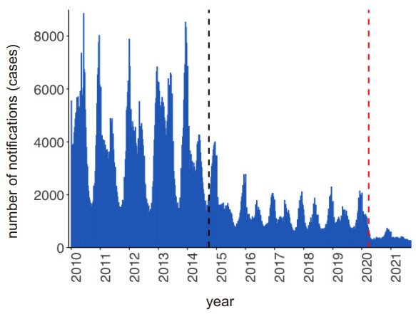
Public health and social measures (PHSMs) targeting the coronavirus disease 2019 (COVID-19) pandemic have potentially affected the epidemiological dynamics of endemic infectious diseases. In this study, we investigated the impact of PHSMs for COVID-19, with a particular focus on varicella dynamics in Japan. We adopted the susceptible-infectious-recovered type of mathematical model to reconstruct the epidemiological dynamics of varicella from Jan. 2010 to Sep. 2021. We analyzed epidemiological and demographic data and estimated the within-year and multi-year component of the force of infection and the biases associated with reporting and ascertainment in three periods: pre-vaccination (Jan. 2010–Dec. 2014), pre-pandemic vaccination (Jan. 2015–Mar. 2020) and during the COVID-19 pandemic (Apr. 2020–Sep. 2021). By using the estimated parameter values, we reconstructed and predicted the varicella dynamics from 2010 to 2027. Although the varicella incidence dropped drastically during the COVID-19 pandemic, the change in susceptible dynamics was minimal; the number of susceptible individuals was almost stable. Our prediction showed that the risk of a major outbreak in the post-pandemic era may be relatively small. However, uncertainties, including age-related susceptibility and travel-related cases, exist and careful monitoring would be required to prepare for future varicella outbreaks.
- chickenpox,
- SARS-CoV-2,
- mathematical model,
- COVID-19 pandemic,
- immunization
Citation: Ayako Suzuki, Hiroshi Nishiura. Transmission dynamics of varicella before, during and after the COVID-19 pandemic in Japan: a modelling study[J]. Mathematical Biosciences and Engineering, 2022, 19(6): 5998-6012. doi: 10.3934/mbe.2022280

Related Papers:

Abstract

Public health and social measures (PHSMs) targeting the coronavirus disease 2019 (COVID-19) pandemic have potentially affected the epidemiological dynamics of endemic infectious diseases. In this study, we investigated the impact of PHSMs for COVID-19, with a particular focus on varicella dynamics in Japan. We adopted the susceptible-infectious-recovered type of mathematical model to reconstruct the epidemiological dynamics of varicella from Jan. 2010 to Sep. 2021. We analyzed epidemiological and demographic data and estimated the within-year and multi-year component of the force of infection and the biases associated with reporting and ascertainment in three periods: pre-vaccination (Jan. 2010–Dec. 2014), pre-pandemic vaccination (Jan. 2015–Mar. 2020) and during the COVID-19 pandemic (Apr. 2020–Sep. 2021). By using the estimated parameter values, we reconstructed and predicted the varicella dynamics from 2010 to 2027. Although the varicella incidence dropped drastically during the COVID-19 pandemic, the change in susceptible dynamics was minimal; the number of susceptible individuals was almost stable. Our prediction showed that the risk of a major outbreak in the post-pandemic era may be relatively small. However, uncertainties, including age-related susceptibility and travel-related cases, exist and careful monitoring would be required to prepare for future varicella outbreaks.

References

[1]	D. Enria, Z. Feng, A. Fretheim, C. Ihekweazu, T. Ottersen, A. Schuchat, et al., Strengthening the evidence base for decisions on public health and social measures, Bull. W. H. O., 99 (2021), 610–610A. https://doi.org/10.2471/BLT.21.287054 doi: 10.2471/BLT.21.287054
[2]	B. J. Cowling, S. T. Ali, T. Ng, T. K. Tsang, J. C. M. Li, M. W. Fong, et al., Impact assessment of non-pharmaceutical interventions against coronavirus disease 2019 and influenza in Hong Kong: an observational study, Lancet Public Health, 5 (2020), E279–E288. https://doi.org/10.1016/S2468-2667(20)30090-6 doi: 10.1016/S2468-2667(20)30090-6
[3]	S. G. Sullivan, S. Carlson, A. C. Cheng, M. B. Chilver, D. E. Dwyer, M. Irwin, et al., Where has all the influenza gone? The impact of COVID-19 on the circulation of influenza and other respiratory viruses, Australia, March to September 2020, Eurosurveillance, 25 (2020). https://doi.org/10.2807/1560-7917.ES.2020.25.47.2001847 doi: 10.2807/1560-7917.ES.2020.25.47.2001847
[4]	S. J. Olsen, A. K. Winn, A. P. Budd, M. M. Prill, J. Steel, C. M. Midgley, et al., Changes in influenza and other respiratory virus activity during the COVID-19 pandemic–United States, 2020–2021, Morb. Mortal. Wkly. Rep., 70 (2021), 1013–1019. https://doi.org/10.15585/mmwr.mm7029a1 doi: 10.15585/mmwr.mm7029a1
[5]	National Institute of Infectious Diseases, Tuberculosis and Infectious Diseases Department, Health Service Bureau, Ministry of Health, Labour and Welfare. Infect. Agents Surveill. Rep. (IASR), 42 (2021), 239–270. Available from: https://www.niid.go.jp/niid/images/idsc/iasr/42/501.pdf.
[6]	National Institute of Infectious Diseases, Tuberculosis and Infectious Diseases Department, Health Service Bureau, Ministry of Health, Labour and Welfare. Infect. Dis. Wkly. Rep. (IDWR), 23 (2021), 29. Available from: https://www.niid.go.jp/niid/images/idsc/idwr/IDWR2021/idwr2021-29.pdf.
[7]	R. E. Baker, S. W. Park, W. Yang, G. A. Vecchi, C. J. E. Metcalf, B. T. Grenfell, The impact of COVID-19 nonpharmaceutical interventions on the future dynamics of endemic infections, Proc. Natl. Acad. Sci., 117 (2020), 30547–30553. https://doi.org/10.1073/pnas.2013182117 doi: 10.1073/pnas.2013182117
[8]	L. Madaniyazi, X. Seposo, C. F. S. Ng, A. Tobias, M. Toizumi, H. Moriuchi, et al., Respiratory syncytial virus outbreaks are predicted after the COVID-19 pandemic in Tokyo, Japan, Jpn. J. Infect. Dis., 75 (2022), 209–211. https://doi.org/10.7883/yoken.JJID.2021.312 doi: 10.7883/yoken.JJID.2021.312
[9]	M. Ujiie, S. Tsuzuki, T. Nakamoto, N. Iwamoto, Resurgence of respiratory syncytial virus infections during COVID-19 pandemic, Tokyo, Japan, Emerging Infect. Dis., 27 (2021), 2969–2970. https://doi.org/10.3201/eid2711.211565 doi: 10.3201/eid2711.211565
[10]	A. A. Gershon, J. Breuer, J. I. Cohen, R. J. Cohrs, M. D. Gershon, D. Gilfen, et al., Varicella zoster virus infection, Nat. Rev. Dis. Primers, 1 (2015), 15016. https://doi.org/10.1038/nrdp.2015.16 doi: 10.1038/nrdp.2015.16
[11]	WHO Vaccine-Preventable Diseases: Monitoring System 2018, World Health Organization.
[12]	M. Marin, M. Marti, A. Kambhampati, S. M. Jeram, J. F. Seward, Global varicella vaccine effectiveness: A meta-analysis, Pediatrics, 137 (2016), e20153741. https://doi.org/10.1542/peds.2015-3741 doi: 10.1542/peds.2015-3741
[13]	M. E. Halloran, S. L. Cochi, T. A. Lieu, M. Wharton, L. Fehrs, Theoretical epidemiologic and morbidity effects of routine varicella immunization of preschool children in the United States, Am. J. Epidemiol., 140 (1994), 81–104. https://doi.org/10.1093/oxfordjournals.aje.a117238 doi: 10.1093/oxfordjournals.aje.a117238
[14]	M. Brisson, W. J. Edmunds, N. J. Gay, B. Law, G. D. Serres, Modelling the impact of immunization on the epidemiology of varicella zoster virus, Epidemiol. Infect., 125 (2000), 651–669. https://doi.org/10.1017/S0950268800004714 doi: 10.1017/S0950268800004714
[15]	H. F. Gidding, M. Brisson, C. R. Macintyre, M. A. Burgess, Modelling the impact of vaccination on the epidemiology of varicella zoster virus in Australia, Aust. N. Z. J. Public Health, 29 (2005), 544–551. https://doi.org/10.1111/j.1467-842X.2005.tb00248.x doi: 10.1111/j.1467-842X.2005.tb00248.x
[16]	Z. Gao, H. F. Gidding, J. G. Wood, C. R. MacIntyre, Modelling the impact of one-dose vs. two-dose vaccination regimens on the epidemiology of varicella zoster virus in Australia, Epidemiol. Infect., 138 (2010), 457–468. https://doi.org/10.1017/S0950268809990860 doi: 10.1017/S0950268809990860
[17]	M. Karhunen, T. Leino, H. Salo, I. Davidkin, T. Kilpi, K. Auranen, Modelling the impact of varicella vaccination on varicella and zoster, Epidemiol. Infect., 138 (2010), 469–481. https://doi.org/10.1017/S0950268809990768 doi: 10.1017/S0950268809990768
[18]	A. J. V. Hoek, A. Melegaro, E. Zagheni, W. J. Edmunds, N. Gay, Modelling the impact of a combined varicella and zoster vaccination programme on the epidemiology of varicella zoster virus in England, Vaccine, 29 (2011), 2411–2420. https://doi.org/10.1016/j.vaccine.2011.01.037 doi: 10.1016/j.vaccine.2011.01.037
[19]	A. Melegaro, V. Marziano, E. D. Fava, P. Poletti, M. Tirani, C. Rizzo, et al., The impact of demographic changes, exogenous boosting and new vaccination policies on varicella and herpes zoster in Italy: A modelling and cost-effectiveness study, BMC Med., 16 (2018), 117. https://doi.org/10.1186/s12916-018-1094-7 doi: 10.1186/s12916-018-1094-7
[20]	J. Karsai, R. Csuma-Kovács, Å. Dánielisz, Z. Molnár, J. Dudás, T. Borsos, et al., Modeling the transmission dynamics of varicella in Hungary, J. Math. Ind., 10 (2020), 12. https://doi.org/10.1186/s13362-020-00079-z doi: 10.1186/s13362-020-00079-z
[21]	J. Suh, T. Lee, J. K. Choi, J. Lee, S. H. Park, The impact of two-dose varicella vaccination on varicella and herpes zoster incidence in South Korea using a mathematical model with changing population demographics, Vaccine., 39 (2021), 2575–2583. https://doi.org/10.1016/j.vaccine.2021.03.056 doi: 10.1016/j.vaccine.2021.03.056
[22]	M. Pawaskar, C. Burgess, M. Pillsbury, T. Wisløff, E. Flem, Clinical and economic impact of universal varicella vaccination in Norway: a modeling study, PLoS One, 16 (2021), e0254080. https://doi.org/10.1371/journal.pone.0254080 doi: 10.1371/journal.pone.0254080
[23]	National Institute of Infectious Diseases, Tuberculosis and Infectious Diseases Department, Health Service Bureau, Ministry of Health, Labour and Welfare, Cumulative vaccination coverage report. Available from: https://www.niid.go.jp/niid/images/vaccine/cum-vaccine-coverage/cum-vaccine-coverage_30.pdf.
[24]	A. Suzuki, H. Nishiura, Reconstructing the transmission dynamics of varicella in Japan: An elevation of age at infection, PeerJ, 10 (2022), e12767. https://doi.org/10.7717/peerj.12767 doi: 10.7717/peerj.12767
[25]	Ministry of Health, Labour and Welfare of Japan. 2021a. Notification rules of infectious diseases: Chickenpox. Available from: https://www.mhlw.go.jp/bunya/kenkou/kekkaku-kansenshou11/01-05-19.html.
[26]	Infectious Disease Surveillance Center, The report of national epidemiological surveillance of vaccine-preventable diseases. Available form: https://www.niid.go.jp/niid/ja/y-reports/669-yosoku-report.html.
[27]	T. Ozaki, Long-term clinical studies of varicella vaccine at a regional hospital in Japan and proposal for a varicella vaccination program, Vaccine, 31 (2013), 6155–6160. https://doi.org/10.1016/j.vaccine.2013.10.060 doi: 10.1016/j.vaccine.2013.10.060
[28]	National Institute of Population and Social Security Research, Population projections for Japan (2017): 2016 to 2065. Available from: http://www.ipss.go.jp/pp-zenkoku/e/zenkoku_e2017/pp29_summary.pdf.
[29]	P. E. Fine, J. A. Clarkson, Measles in England and Wales–I: An analysis of factors underlying seasonal patterns, Int. J. Epidemiol., 11 (1982), 5–14. https://doi.org/10.1093/ije/11.1.5 doi: 10.1093/ije/11.1.5

Reader Comments

Your name:*

Email:*
© 2022 the Author(s), licensee AIMS Press. This is an open access article distributed under the terms of the Creative Commons Attribution License (http://creativecommons.org/licenses/by/4.0)