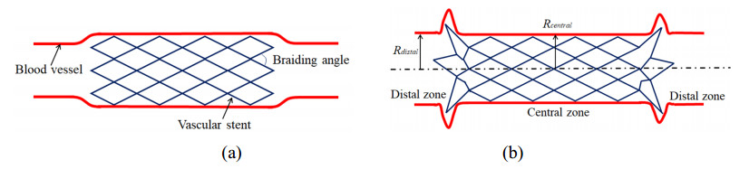
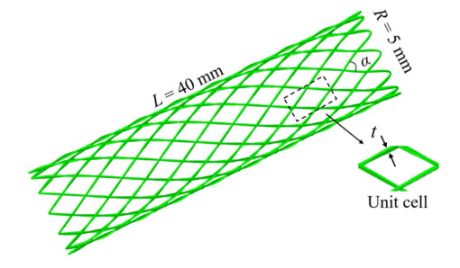
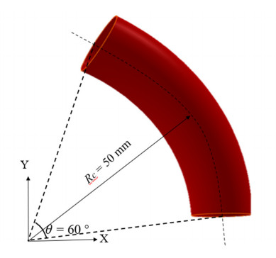
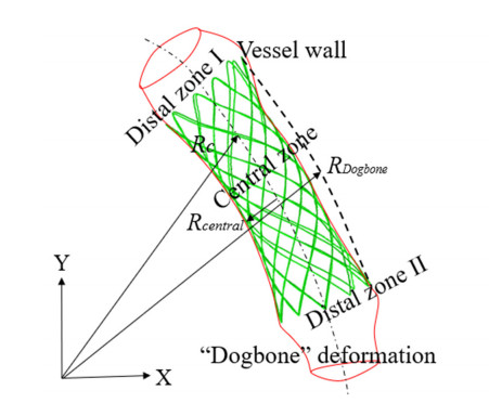
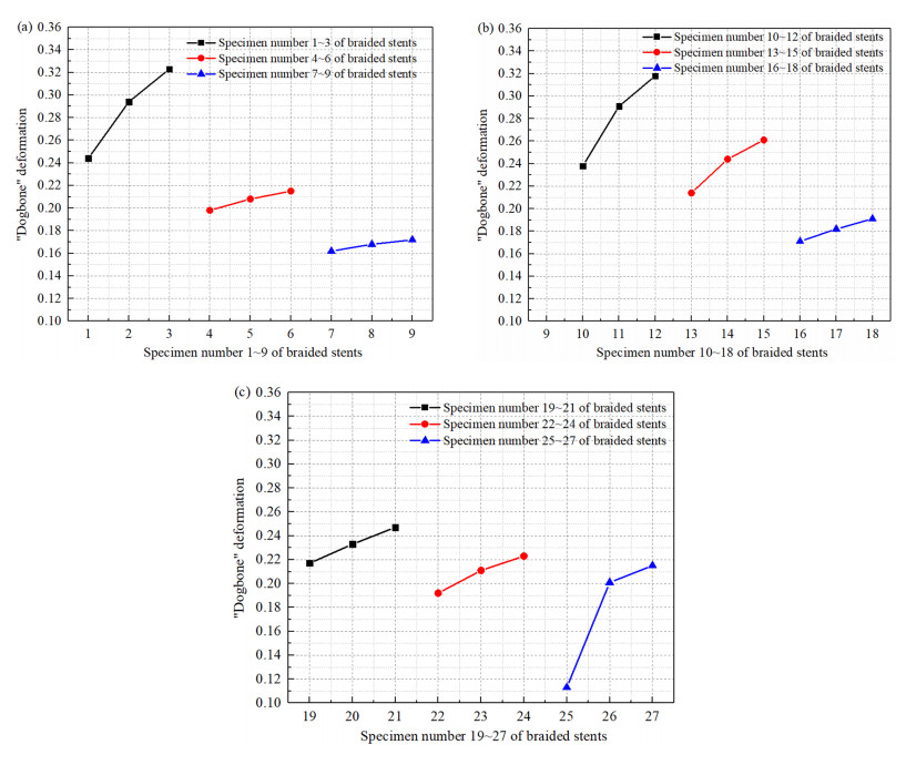
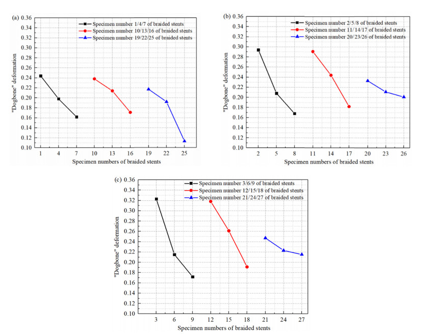
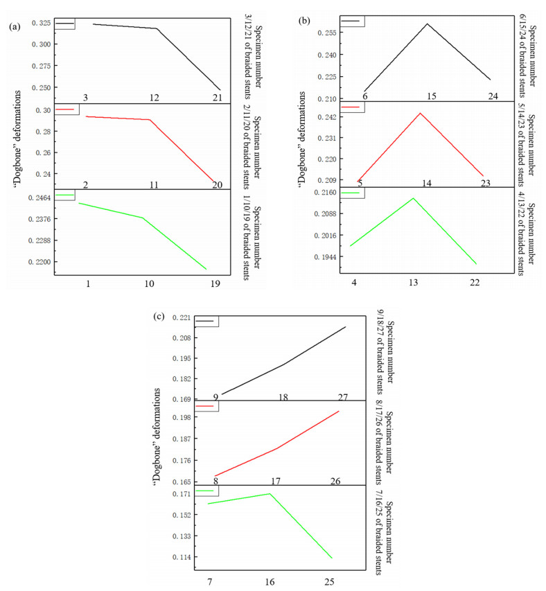
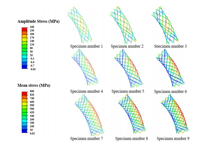
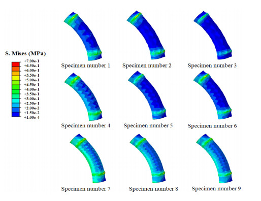
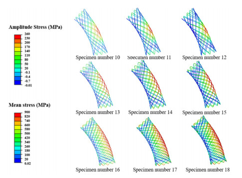
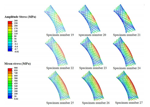
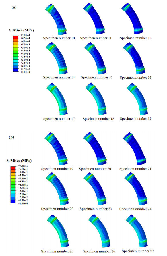
"Dogbone" deformation that the diameters of two ends are larger than the middle diameter of the stent under the effect of the balloon expanding, is one of the important standards to evaluate the mechanical properties of vascular stents. It is a huge challenge to simulate and evaluate the "Dogbone" behaviors of braided stents in the curved vessels. In this study, the key work was to investigate the "Dogbone" deformations of braided stents in the curved vessels by designing main parameters including strut diameter, braiding angle, and the circumferential number of unit cell. Based on the "Dogbone" stents in the curved vessels, the impact of "Dogbone" on the fatigue properties of braided stents was analyzed under the pulsatile effect of vessels. The influence of "Dogbone" stents on stress distribution of vascular walls was studied. To evaluate the "Dogbone" behaviors of stents in the curved vessels, the calculation method of "Dogbone" was improved by calculating the centerline and the bus bar of the curved vessels. Braided stents with various parameters (strut diameter t = 100,125 and 152 μm, braiding angle α = 30, 40 and 50°, the circumferential number of unit cell N = 8, 10, and 12) were designed respectively. Numerical simulation method was used to mimic the "Dogbone" deformation after stent expansion. The results showed that strut diameter and braiding angle had more influence on "Dogbone" deformations than the circumferential number of unit cell. "Dogbone" deformation could adversely affect fatigue performance and vascular walls.
Citation: Chen Pan, Xinyun Zeng, Yafeng Han, Jiping Lu. Investigation of braided stents in curved vessels in terms of "Dogbone" deformation[J]. Mathematical Biosciences and Engineering, 2022, 19(6): 5717-5737. doi: 10.3934/mbe.2022267
"Dogbone" deformation that the diameters of two ends are larger than the middle diameter of the stent under the effect of the balloon expanding, is one of the important standards to evaluate the mechanical properties of vascular stents. It is a huge challenge to simulate and evaluate the "Dogbone" behaviors of braided stents in the curved vessels. In this study, the key work was to investigate the "Dogbone" deformations of braided stents in the curved vessels by designing main parameters including strut diameter, braiding angle, and the circumferential number of unit cell. Based on the "Dogbone" stents in the curved vessels, the impact of "Dogbone" on the fatigue properties of braided stents was analyzed under the pulsatile effect of vessels. The influence of "Dogbone" stents on stress distribution of vascular walls was studied. To evaluate the "Dogbone" behaviors of stents in the curved vessels, the calculation method of "Dogbone" was improved by calculating the centerline and the bus bar of the curved vessels. Braided stents with various parameters (strut diameter t = 100,125 and 152 μm, braiding angle α = 30, 40 and 50°, the circumferential number of unit cell N = 8, 10, and 12) were designed respectively. Numerical simulation method was used to mimic the "Dogbone" deformation after stent expansion. The results showed that strut diameter and braiding angle had more influence on "Dogbone" deformations than the circumferential number of unit cell. "Dogbone" deformation could adversely affect fatigue performance and vascular walls.

| [1] |
R. W. Günther, D. Vorwerk, K. Bohndorf, K. C. Klose, D. Kistler, H. Mann, et al., Venous stenoses in dialysis shunts: Treatment with self-expanding metallic stents, Radiology, 170 (1989), 401-405. https://doi.org/10.1148/radiology.170.2.2521397 doi: 10.1148/radiology.170.2.2521397

|
| [2] |
C. G. Mckenna, T. J. Vaughan, An experimental evaluation of the mechanics of bare and polymer-covered self-expanding wire braided stents, J. Mech. Behav. Biomed. Mater., 103 (2020), 103549. https://doi.org/10.1016/j.jmbbm.2019.103549 doi: 10.1016/j.jmbbm.2019.103549
|
| [3] |
C. G. Mckenna, T. J. Vaughan. A finite element investigation on design parameters of bare and polymer-covered self-expanding wire braided stents, J. Mech. Behav. Biomed. Mater., 115 (2021), 104305. https://doi.org/10.1016/j.jmbbm.2020.104305 doi: 10.1016/j.jmbbm.2020.104305
|
| [4] |
K. C. Ueng, S. P. Wen, C. W. Lou, J. H. Lin. Stainless steel/nitinol braid coronary stents: Braiding structure stability and cut section treatment evaluation, J. Ind. Text., 45 (2016), 965-977. https://doi.org/10.1177/1528083714550054 doi: 10.1177/1528083714550054
|
| [5] |
Q. Zheng, H. Mozafari, Z. Li, L. Gu, M. An, X. Han, et al., Mechanical characterization of braided self-expanding stents: Impact of design parameters, J. Mech. Med. Biol., 19 (2019), 1950038. https://doi.org/10.1142/S0219519419500386 doi: 10.1142/S0219519419500386
|
| [6] |
F. Zhao, W. Xue, F. Wang, J. Sun, J. Lin, L. Liu, et al., Braided bioresorbable cardiovascular stents mechanically reinforced by axial runners, J. Mech. Behav. Biomed. Mater., 89 (2019), 19-32. https://doi.org/10.1016/j.jmbbm.2018.09.003 doi: 10.1016/j.jmbbm.2018.09.003
|
| [7] |
J. Sun, K. Sun, K. Bai, S. Chen, F. J. Wang, F. Zhao, et al., A novel braided biodegradable stent for use in congenital heart disease: Short-term results in porcine iliac artery, J. Biomed. Mater. Res. A, 107 (2019), 1667-1677. https://doi.org/10.1002/jbm.a.36682 doi: 10.1002/jbm.a.36682
|
| [8] |
C. Shanahan, P. Tiernan, S. A. M. Tofail, Looped ends versus open ends braided stent: A comparison of the mechanical behaviour using analytical and numerical methods, J. Mech. Behav. Biomed. Mater., 75 (2017), 581-591. https://doi.org/10.1016/j.jmbbm.2017.08.025 doi: 10.1016/j.jmbbm.2017.08.025
|
| [9] |
H. Zahedmanesh, D. John Kelly, C. Lally, Simulation of a balloon expandable stent in a realistic coronary artery-determination of the optimum modelling strategy, J. Biomech., 43 (2010), 2126-2132. https://doi.org/10.1016/j.jbiomech.2010.03.050 doi: 10.1016/j.jbiomech.2010.03.050
|
| [10] |
L. Wei, Q. Chen, Z. Li, Study on the impact of straight stents on arteries with different curvatures, J. Mech. Med. Biol., 16 (2016), 1-13. https://doi.org/10.1142/S0219519416500937 doi: 10.1142/S0219519416500937
|
| [11] |
L. Wei, H. L. Leo, Q. Chen, Z. Li, Structural and hemodynamic analyses of different stent structures in curved and stenotic coronary artery, Front Bioeng. Biotechnol., 7 (2019), 1-13. https://doi.org/10.3389/fbioe.2019.00366 doi: 10.3389/fbioe.2019.00366
|
| [12] |
W. Wu, W. Q. Wang, D. Z. Yang, M. Qi, Stent expansion in curved vessel and their interactions: A finite element analysis, J. Biomech., 40 (2007), 2580-2585. https://doi.org/10.1016/j.jbiomech.2006.11.009 doi: 10.1016/j.jbiomech.2006.11.009
|
| [13] |
S. Kasiri, D. J. Kelly, An argument for the use of multiple segment stents in curved arteries, J. Biomech. Eng., 133 (2011), 2-6. https://doi.org/10.1115/1.4004863 doi: 10.1115/1.4004863
|
| [14] |
Y. Han, W. Lu, Optimizing the deformation behavior of stent with nonuniform Poisson's ratio distribution for curved artery, J. Mech. Behav. Biomed. Mater., 88 (2018), 442-452. https://doi.org/10.1016/j.jmbbm.2018.09.005 doi: 10.1016/j.jmbbm.2018.09.005
|
| [15] |
J. A. Ormiston, S. R. Dixon, M. W. I. Webster, P. N. Ruygrok, J. T. Stewart, I. Min-chington, et al., Stent longitudinal flexibility: A comparison of 13 stent designs before and after balloon expansion, Catheter Cardiovasc. Interv., 50 (2000), 120-124. https://doi.org/10.1002/(SICI)1522-726X(200005)50:1<120::AID-CCD26>3.0.CO;2-T doi: 10.1002/(SICI)1522-726X(200005)50:1<120::AID-CCD26>3.0.CO;2-T
|
| [16] |
B. P. Murphy, P. Savage, P. E. McHugh, D. F. Quinn, The stress-strain behavior of cor-onary stent struts is size dependent, Ann. Biomed. Eng., 31 (2003), 686-691. https://doi.org/10.1114/1.1569268 doi: 10.1114/1.1569268
|
| [17] |
R. Rieu, P. Barragan, V. Garitey, P. O. Roquebert, J. Fuseri, P. Commeau, et al., Assessment of the trackability, flexibility, and conformability of coronary stents: A comparative analysis, Catheter Cardiovasc. Interv., 59 (2003), 496-503. https://doi.org/10.1002/ccd.10583 doi: 10.1002/ccd.10583
|
| [18] |
K. Mori, T. Saito, Effects of stent structure on stent flexibility measurements, Ann. Biomed. Eng., 33 (2005), 733-742. https://doi.org/10.1007/s10439-005-2807-6 doi: 10.1007/s10439-005-2807-6
|
| [19] |
S. Pant, G. Limbert, N. P. Curzen, N. W. Bressloff, Multiobjective design optimisation of coronary stents, Biomaterials, 32 (2011), 7755-7773. https://doi.org/10.1016/j.biomaterials.2011.07.059 doi: 10.1016/j.biomaterials.2011.07.059
|
| [20] |
S. Tammareddi, G. Sun, Q. Li, Multiobjective robust optimization of coronary stents, Mater. Des., 90 (2016), 682-692. https://doi.org/10.1016/j.matdes.2015.10.153 doi: 10.1016/j.matdes.2015.10.153
|
| [21] |
J. Raamachandran, K. Jayavenkateshwaran, Modeling of stents exhibiting negative Poisso-n's ratio effect, Comput. Methods Biomech. Biomed. Eng., 10 (2007), 245-255. https://doi.org/10.1080/10255840701198004 doi: 10.1080/10255840701198004
|
| [22] |
P. K. M. Prithipaul, M. Kokkolaras, D. Pasini, Assessment of structural and hemodynamic performance of vascular stents modelled as periodic lattices, Med. Eng. Phys., 57 (2018), 11-18. https://doi.org/10.1016/j.medengphy.2018.04.017 doi: 10.1016/j.medengphy.2018.04.017
|
| [23] |
K. Maleckis, P. Deegan, W. Poulson, C. Sievers, A. Desyatova, J. MacTaggart, et al., Comparison of femoropopliteal artery stents under axial and radial compression, axial tension, bending, and torsion deformations, J. Mech. Behav. Biomed. Mater., 75 (2017), 160-168. https://doi.org/10.1016/j.jmbbm.2017.07.017 doi: 10.1016/j.jmbbm.2017.07.017
|
| [24] |
M. De Beule, P. Mortier, S. G. Carlier, B. Verhegghe, R. Van Impe, P. Verdonck, Realistic finite element-based stent design: The impact of balloon folding, J. Biomech., 41 (2008), 383-389. https://doi.org/10.1016/j.jbiomech.2007.08.014 doi: 10.1016/j.jbiomech.2007.08.014
|
| [25] |
G. R. Douglas, S. A. Phani, J. Gagnon, Analyses and design of expansion mechanisms of balloon expandable vascular stents, J. Biomech., 47 (2014), 1438-1446. https://doi.org/10.1016/j.jbiomech.2014.01.039 doi: 10.1016/j.jbiomech.2014.01.039
|
| [26] |
W. Q. Wang, D. K. Liang, D. Z. Yang, M. Qi, Analysis of the transient expansion behavior and design optimization of coronary stents by finite element method, J. Biomech., 39 (2006), 21-32. https://doi.org/10.1016/j.jbiomech.2004.11.003 doi: 10.1016/j.jbiomech.2004.11.003
|
| [27] |
A. Giuliodori, J. A. Hernández, D. Fernandez-Sanchez, I. Galve, E. Soudah, Numerical modeling of bare and polymer-covered braided stents using torsional and tensile springs connectors, J. Biomech., 123 (2021), 110459. https://doi.org/10.1016/j.jbiomech.2021.110459 doi: 10.1016/j.jbiomech.2021.110459
|
| [28] |
Z. Liu, L. Wu, J. Yang, F. Cui, G. Chen, Thoracic aorta stent grafts design in terms of biomechanical investigations into flexibility, Math. Biosci. Eng., 18 (2020), 800-816. https://doi.org/10.3934/mbe.2021042 doi: 10.3934/mbe.2021042
|
| [29] | M. Azaouzi, A. Makradi, S. Belouettar, Numerical investigations of the structural behavior of a balloon expandable stent design using finite element method, Comput. Mater. Sci., 72 (2013), 54-61. https://doi.org/doi:10.1016/j.commatsci.2013.01.031 |
| [30] |
Z. Y. Zhang, An experimental and theoretical study on the anisotropy of elastin network, Ann. Biomed. Eng., 37 (2009), 1572-1583. https://doi.org/10.1007/s10439-009-9724-z doi: 10.1007/s10439-009-9724-z
|
| [31] |
G. A. Holzapfel, G. Sommer, C. T. Gasser, P. Regitnig, Determination of layer-specific mechanical properties of human coronary arteries with nonatherosclerotic intimal thickening and related constitutive modeling, Am. J. Physiol. Heart Circ. Physiol., 289 (2005), H2048. https://doi.org/10.1152/ajpheart.00934.2004 doi: 10.1152/ajpheart.00934.2004
|
| [32] |
M. Umer, M. N. Ali, A. Mubashar, M. Mir, Computational modeling of balloon-expandable stent deployment in coronary artery using the finite element method, Res. Rep. Clin. Cardiol., 10 (2019), 43-56. https://doi.org/10.2147/rrcc.s173086 doi: 10.2147/rrcc.s173086
|
| [33] |
A. Schiavone, L. G. Zhao, A study of balloon type, system constraint and artery constitutive model used in finite element simulation of stent deployment, Mech. Adv. Mater. Mod. Process, 1 (2015), 1-15. https://doi.org/10.1186/s40759-014-0002-x doi: 10.1186/s40759-014-0002-x
|
| [34] |
H. Zahedmanesh, C. Lally, Determination of the influence of stent strut thickness using the finite element method: Implications for vascular injury and in-stent restenosis, Med. Biol. Eng. Comput., 47 (2009), 385-393. https://doi.org/10.1007/s11517-009-0432-5 doi: 10.1007/s11517-009-0432-5
|
| [35] |
F. Migliavacca, L. Petrini, M. Colombo, F. Auricchio, R. Pietrabissa, Mechanical behavior of coronary stents investigated through the finite element method, J. Biomech., 35 (2002), 803-811. https://doi.org/10.1016/S0021-9290(02)00033-7 doi: 10.1016/S0021-9290(02)00033-7
|
| [36] |
M. Azaouzi, A. Makradi, S. Belouettar, Deployment of a self-expanding stent inside an artery: A finite element analysis, Mater. Des., 41 (2012), 410-420. https://doi.org/10.1016/j.matdes.2012.05.019 doi: 10.1016/j.matdes.2012.05.019
|
| [37] |
L. Lei, X. Qi, S. Li, Y. Yang, Y. Hu, B. Li, et al., Finite element analysis for fatigue behaviour of a self-expanding Nitinol peripheral stent under physiological biomechanical conditions, Comput. Biol. Med., 104 (2019), 205-214. https://doi.org/10.1016/j.compbiomed.2018.11.019 doi: 10.1016/j.compbiomed.2018.11.019
|
| [38] |
G. Praveen Kumar, A. Louis Commillus, F. Cui, A finite element simulation method to evaluate the crimpability of curved stents, Med. Eng. Phys., 74 (2019), 162-165. https://doi.org/10.1016/j.medengphy.2019.07.017 doi: 10.1016/j.medengphy.2019.07.017
|
| [39] |
L. Petrini, W. Wu, E. Dordoni, A. Meoli, F. Migliavacca, G. Pennati, Fatigue behavior characterization of nitinol for peripheral stents, Funct. Mater. Lett., 5 (2012), 1250012. https://doi.org/10.1142/S1793604712500129 doi: 10.1142/S1793604712500129
|
| [40] |
A. Meoli, E. Dordoni, L. Petrini, F. Migliavacca, G. Dubini, G. Pennati, Computational modelling of in vitro set-ups for peripheral self-expanding nitinol stents: the importance of stent-wall interaction in the assessment of the fatigue resistance, Cardiovasc. Eng. Technol., 4 (2013), 474-484. https://doi.org/10.1007/s13239-013-0164-4 doi: 10.1007/s13239-013-0164-4
|
| [41] |
A. Meoli, E. Dordoni, L. Petrini, F. Migliavacca, G. Dubini, G. Pennati, Computational study of axial fatigue for peripheral nitinol stents, J. Mater. Eng. Perform., 23 (2014), 2606-2613. https://doi.org/10.1007/s11665-014-0965-0 doi: 10.1007/s11665-014-0965-0
|
| [42] | S. Gopal, S. Kim, R. Swift, B. Choules, Fatigue life estimation of nitinol medical devices, Strain, (2008), 1-10. |
| [43] |
D. Elena, P. Lorenza, W. Wei, M. Francesco, D. Gabriele, P. Giancarlo, Computational modeling to predict fatigue behavior of NiTi stents: What do we need? J. Funct. Biomater., 6 (2015), 299-317. https://doi.org/10.3390/jfb6020299 doi: 10.3390/jfb6020299
|
| [44] |
C. Shanahan, S. Tofail, P. Tiernan, Viscoelastic braided stent: finite element analysis and validation of crimping behaviour, Mater. Design, 121 (2017), 143-153. https://doi.org/10.1016/j.matdes.2017.02.044 doi: 10.1016/j.matdes.2017.02.044
|
| [45] |
J. H. Kim, T. J. Kang, W. R. Yu, Simulation of mechanical behavior of temperature-responsive braided stents made of shape memory polyurethanes, J. Biomech., 43 (2010), 632-643. https://doi.org/10.1016/j.jbiomech.2009.10.032 doi: 10.1016/j.jbiomech.2009.10.032
|
Figures(12) / Tables(6)

Chen Pan, Xinyun Zeng, Yafeng Han, Jiping Lu. Investigation of braided stents in curved vessels in terms of "Dogbone" deformation[J]. Mathematical Biosciences and Engineering, 2022, 19(6): 5717-5737. doi: 10.3934/mbe.2022267


 DownLoad: