Classifying and identifying surface defects is essential during the production and use of aluminum profiles. Recently, the dual-convolutional neural network(CNN) model fusion framework has shown promising performance for defects classification and recognition. Spurred by this trend, this paper proposes an improved dual-CNN model fusion framework to classify and identify defects in aluminum profiles. Compared with traditional dual-CNN model fusion frameworks, the proposed architecture involves an improved fusion layer, fusion strategy, and classifier block. Specifically, the suggested method extracts the feature map of the aluminum profile RGB image from the pre-trained VGG16 model's pool5 layer and the feature map of the maximum pooling layer of the suggested A4 network, which is added after the Alexnet model. then, weighted bilinear interpolation unsamples the feature maps extracted from the maximum pooling layer of the A4 part. The network layer and upsampling schemes ensure equal feature map dimensions ensuring feature map merging utilizing an improved wavelet transform. Finally, global average pooling is employed in the classifier block instead of dense layers to reduce the model's parameters and avoid overfitting. The fused feature map is then input into the classifier block for classification. The experimental setup involves data augmentation and transfer learning to prevent overfitting due to the small-sized data sets exploited, while the K cross-validation method is employed to evaluate the model's performance during the training process. The experimental results demonstrate that the proposed dual-CNN model fusion framework attains a classification accuracy higher than current techniques, and specifically 4.3% higher than Alexnet, 2.5% for VGG16, 2.9% for Inception v3, 2.2% for VGG19, 3.6% for Resnet50, 3% for Resnet101, and 0.7% and 1.2% than the conventional dual-CNN fusion framework 1 and 2, respectively, proving the effectiveness of the proposed strategy.
Citation: Xiaochen Liu, Weidong He, Yinghui Zhang, Shixuan Yao, Ze Cui. Effect of dual-convolutional neural network model fusion for Aluminum profile surface defects classification and recognition[J]. Mathematical Biosciences and Engineering, 2022, 19(1): 997-1025. doi: 10.3934/mbe.2022046
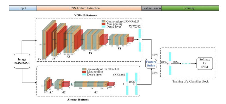
Classifying and identifying surface defects is essential during the production and use of aluminum profiles. Recently, the dual-convolutional neural network(CNN) model fusion framework has shown promising performance for defects classification and recognition. Spurred by this trend, this paper proposes an improved dual-CNN model fusion framework to classify and identify defects in aluminum profiles. Compared with traditional dual-CNN model fusion frameworks, the proposed architecture involves an improved fusion layer, fusion strategy, and classifier block. Specifically, the suggested method extracts the feature map of the aluminum profile RGB image from the pre-trained VGG16 model's pool5 layer and the feature map of the maximum pooling layer of the suggested A4 network, which is added after the Alexnet model. then, weighted bilinear interpolation unsamples the feature maps extracted from the maximum pooling layer of the A4 part. The network layer and upsampling schemes ensure equal feature map dimensions ensuring feature map merging utilizing an improved wavelet transform. Finally, global average pooling is employed in the classifier block instead of dense layers to reduce the model's parameters and avoid overfitting. The fused feature map is then input into the classifier block for classification. The experimental setup involves data augmentation and transfer learning to prevent overfitting due to the small-sized data sets exploited, while the K cross-validation method is employed to evaluate the model's performance during the training process. The experimental results demonstrate that the proposed dual-CNN model fusion framework attains a classification accuracy higher than current techniques, and specifically 4.3% higher than Alexnet, 2.5% for VGG16, 2.9% for Inception v3, 2.2% for VGG19, 3.6% for Resnet50, 3% for Resnet101, and 0.7% and 1.2% than the conventional dual-CNN fusion framework 1 and 2, respectively, proving the effectiveness of the proposed strategy.

| [1] |
Z. W. Liu, L. X. Li, J. Yi, S. K. Li, Z. H. Wang, G. Wang, Influence of heat treatment conditions on bending characteristics of 6063 aluminum alloy sheets, T. Nonferr. Metal. Soc., 27 (2017), 1498–1506. doi: 10.1016/s1003-6326(17)60170-5. doi: 10.1016/s1003-6326(17)60170-5

|
| [2] |
S. Bingol, A. Bozaci, Experimental and Numerical Study on the Strength of Aluminum Extrusion Welding, Materials (Basel), 8 (2015), 4389-4399. doi: 10.3390/ma8074389. doi: 10.3390/ma8074389
|
| [3] |
L. Donati, L. Tomesani, The effect of die design on the production and seam weld quality of extruded aluminum profiles, J. Mater. Process. Technol., 164-165 (2005), 1025–1031. doi: 10.1016/j.jmatprotec.2005.02.156. doi: 10.1016/j.jmatprotec.2005.02.156
|
| [4] | C. T. Mgonja, A review on effects of hazards in foundries to workers and environment, IJISET: Int. J. Innov. Sci. Eng. Technol., 4 (2017), 326–334. |
| [5] |
J. Ahmed, B. Gao, W. l. Woo, Sparse low-rank tensor decomposition for metal defect detection using thermographic imaging diagnostics, IEEE T. Ind. Inform., 17 (2020), 1810–1820. doi: 10.1109/TⅡ.2020.2994227. doi: 10.1109/TⅡ.2020.2994227
|
| [6] |
Q. Luo, B. Gao, W. l. Woo, Y. Yang, Temporal and spatial deep learning network for infrared thermal defect detection, NDT & E. Int., 108 (2019), 102164. doi: 10.1016/j.ndteint.2019.102164. doi: 10.1016/j.ndteint.2019.102164
|
| [7] |
B. Z. Hu, B. Gao, W. l. Woo, L. F. Ruan, J. K. Jin, A Lightweight Spatial and Temporal Multi-Feature Fusion Network for Defect Detection, IEEE T. Image Process., 30 (2020), 472–486. doi: 10.1109/TIP.2020.3036770. doi: 10.1109/TIP.2020.3036770
|
| [8] |
J. Ahmed, B. Gao, W. l. Woo, Y. Zhu, Ensemble Joint Sparse Low-Rank Matrix Decomposition for Thermography Diagnosis System, IEEE T. Ind. Electronics, 68 (2020), 2648–2658. doi: 10.1109/TIE.2020.2975484. doi: 10.1109/TIE.2020.2975484
|
| [9] |
J. Sun, C. Li, X. J. Wu, V. Palade, W. Fang, An effective method of weld defect detection and classification based on machine vision, IEEE T. Ind. Inform., 15 (2019), 6322–6333. doi: 10.1109/TⅡ.2019.2896357. doi: 10.1109/TⅡ.2019.2896357
|
| [10] |
Z. F. Zhang, G. R. Wen, S. B. Chen, Weld image deep learning-based on-line defects detection using convolutional neural networks for Al alloy in robotic arc welding, J. Manuf. Process., 45 (2019), 208–216. Doi: 10.1016/j.jmapro.2019.06.023. doi: 10.1016/j.jmapro.2019.06.023
|
| [11] |
Y. Q. Bao, K. C. Song, J. Liu, Y. Y. Wang, Y. H. Yan, H. Yu, et al., Triplet-Graph Reasoning Network for Few-shot Metal Generic Surface Defect Segmentation, IEEE Trans. Instrum. Meas., 70 (2021). doi: 10.1109/TIM.2021.3083561. doi: 10.1109/TIM.2021.3083561
|
| [12] |
S. Fekri-Ershad, F. Tajeripour, Multi-resolution and noise-resistant surface defect detection approach using new version of local binary patterns, Appl. Artif. Intell., 31 (2017), 395–410. doi: 10.1080/08839514.2017.1378012. doi: 10.1080/08839514.2017.1378012
|
| [13] |
P. Y. Jong, C. S. Woosang, K. Gyogwon, S. K. Min, L. Chungki, J. L. Sang, Automated defect inspection system for metal surfaces based on deep learning and data augmentation, J. Manuf. Syst., 55 (2020), 317–324. doi: 10.1016/j.jmsy.2020.03.009. doi: 10.1016/j.jmsy.2020.03.009
|
| [14] |
K. Ihor, M. Pavlo, B. Janette, B. Jakub, Steel surface defect classification using deep residual neural network, Metals, 10 (2020), 846. doi: 10.3390/met10060846. doi: 10.3390/met10060846
|
| [15] |
S. H. Guan, M. Lei, H. Lu, A steel surface defect recognition algorithm based on improved deep learning network model using feature visualization and quality evaluation, IEEE Access, 8 (2020), 49885–49895. doi: 10.1109/ACCESS.2020.2979755. doi: 10.1109/ACCESS.2020.2979755
|
| [16] |
B. Zhang, M. M. Liu, Y. Z. Tian, G. Wu, X. H. Yang, S. Y. Shi, et al., Defect inspection system of nuclear fuel pellet end faces based on machine vision, J. Nucl. Sci. Technol., 57 (2020), 617–623. doi: 10.1080/00223131.2019.1708827. doi: 10.1080/00223131.2019.1708827
|
| [17] |
Z. H. Liu, H. B. Shi, X. F. Zhou, Aluminum Profile Type Recognition Based on Texture Features, Appl. Mech. Mater., 556–562 (2014), 2846–2851. doi: 10.4028/www.scientific.net/AMM.556-562.2846. doi: 10.4028/www.scientific.net/AMM.556-562.2846
|
| [18] |
A. Chondronasios, I. Popov, I, Jordanov., Feature selection for surface defect classification of extruded aluminum profiles, Int. J. Adv. Manuf. Technol., 83 (2015), 33–41. doi: 10.1007/s00170-015-7514-3. doi: 10.1007/s00170-015-7514-3
|
| [19] | A. Krizhevsky, I. Sutskever, G. E. Hinton, ImageNet classification with deep convolutional neural networks, Commun. ACM, 60 (2017), 84–90. |
| [20] |
Q. H. Li, D. Liu, Aluminum Plate Surface Defects Classification Based on the BP Neural Network, Appl. Mech. Mater., 734 (2015), 543–547. doi: 10.4028/www.scientific.net/AMM.734.543. doi: 10.4028/www.scientific.net/AMM.734.543
|
| [21] |
R. F. Wei, Y. B. Bi, Research on Recognition Technology of Aluminum Profile Surface Defects Based on Deep Learning, Materials (Basel), 12 (2019), 1681. doi: 10.3390/ma12101681. doi: 10.3390/ma12101681
|
| [22] |
F. M. Neuhauser, G. Bachmann, P. Hora, Surface defect classification and detection on extruded aluminum profiles using convolutional neural networks, Int. J. Mater. Form., 13 (2019), 591–603. doi: 10.1007/s12289-019-01496-1. doi: 10.1007/s12289-019-01496-1
|
| [23] |
D. F. Zhang, K. C. Song, J. Xu, Y. He, Y. H. Yan, Unified detection method of aluminium profile surface defects: Common and rare defect categories, Opt. Lasers Eng., 126 (2020), 105936. doi: 10.1016/j.optlaseng.2019.105936. doi: 10.1016/j.optlaseng.2019.105936
|
| [24] |
R. X. Chen, D. Y. Cai, X. L. Hu, Z. Zhan, S. Wang, Defect Detection Method of Aluminum Profile Surface Using Deep Self-Attention Mechanism under Hybrid Noise Conditions, IEEE Trans. Instrum. Meas., (2021). doi: 10.1109/TIM.2021.3109723. doi: 10.1109/TIM.2021.3109723
|
| [25] |
J. Liu, K. C. Song, M. Z. Feng, Y. H. Yan, Z. B. Tu, L. Liu, Semi-supervised anomaly detection with dual prototypes autoencoder for industrial surface inspection, Opt. Lasers Eng., 136 (2021), 106324. doi: 10.1016/j.optlaseng.2020.106324. doi: 10.1016/j.optlaseng.2020.106324
|
| [26] |
C. M. Duan, T. C. Zhang, Two-Stream Convolutional Neural Network Based on Gradient Image for Aluminum Profile Surface Defects Classification and Recognition, IEEE Access, 8 (2020), 172152-172165. doi: 10.1109/ACCESS.2020.3025165. doi: 10.1109/ACCESS.2020.3025165
|
| [27] |
Y. L. Yu, F. X. Liu, A Two-Stream Deep Fusion Framework for High-Resolution Aerial Scene Classification, Comput. Intell. Neurosci., 2018 (2018), 8639367. doi: 10.1155/2018/8639367. doi: 10.1155/2018/8639367
|
| [28] |
C. Khraief, F. Benzarti, H. Amiri, Elderly fall detection based on multi-stream deep convolutional networks, Multimed. Tools Appl., 79 (2020), 19537–19560. doi: 10.1007/s11042-020-08812-x. doi: 10.1007/s11042-020-08812-x
|
| [29] |
W. Ye, J. Cheng, F. Yang, Y. Xu, Two-Stream Convolutional Network for Improving Activity Recognition Using Convolutional Long Short-Term Memory Networks, IEEE Access, 7 (2019), 67772–67780. doi: 10.1109/ACCESS.2019.2918808. doi: 10.1109/ACCESS.2019.2918808
|
| [30] |
Q. S. Yan, D. Gong, Y. N. Zhang, Two-Stream Convolutional Networks for Blind Image Quality Assessment, IEEE Trans. Image Process., 28 (2019), 2200–2211. doi: 10.1109/TIP.2018.2883741. doi: 10.1109/TIP.2018.2883741
|
| [31] |
T. Zhang, H. Zhang, R. Wang, Y. D. Wu, A new JPEG image steganalysis technique combining rich model features and convolutional neural networks, Math. Biosci. Eng., 16 (2019), 4069–4081. doi: 10.3934/mbe.2019201. doi: 10.3934/mbe.2019201
|
| [32] |
M. Uno, X. H. Han, Y. W. Chen, Comprehensive Study of Multiple CNNs Fusion for Fine-Grained Dog Breed Categorization, 2018 IEEE Int. Sym. Multim. (ISM), (2018), 198–203. doi: 10.1109/ISM.2018.000-7. doi: 10.1109/ISM.2018.000-7
|
| [33] | T. Akilan, Q. J. Wu, H. Zhang, Effect of fusing features from multiple DCNN architectures in image classification, IET Image Process., 12 (2018), 1102–1110. |
| [34] | D. J. Li, H. T. Guo, B. M. Zhang, C. Zhao, D. H. Yu, Double vision full convolution network for object extraction in remote sensing imagery, J. Image Graph., 25 (2020), 0535–0545. |
| [35] | M. Lin, Q. Chen, S. Yan, Network In Network, arXiv preprint arXiv: 1312. 4400(2013). |
| [36] | K. M. He, X. Zhang, S. Q. Ren, J. Sun, Deep residual learning for image recognition, Proc. IEEE confer. Computer vis. Pattern recognit., (2016), 770–778. |
| [37] | C. Szegedy, W. Liu, Y. Q. Jia, P. Sermanet, S. Reed, D. Anguelov, et al., Going deeper with convolutions, Proc. IEEE confer. Computer vis. Pattern recognit., (2015), 1–9. |
| [38] | K. Simonyan, A. Zisserman, Very Deep Convolutional Networks for Large-Scale Image Recognition, arXiv preprint arXiv: 1409. 1556 (2014). |
| [39] | Y. Lecun, Y. Bengio, Convolutional Networks for Images, Speech, and Time-Series, The Handbook of Brain Theory & Neural Networks, 3361 (10), 1995. |
| [40] |
V. Suarez-Paniagua, I. Segura-Bedmar, Evaluation of pooling operations in convolutional architectures for drug-drug interaction extraction, BMC Bioinformatics, 19 (2018), 209. doi: 10.1186/s12859-018-2195-1. doi: 10.1186/s12859-018-2195-1
|
| [41] |
X. L. Zhang, J. F. Xu, J. Yang, L. Chen, H. B. Zhou, X. J. Liu, et al., Understanding the learning mechanism of convolutional neural networks in spectral analysis, Anal Chim Acta, 1119 (2020), 41–51. doi: 10.1016/j.aca.2020.03.055. doi: 10.1016/j.aca.2020.03.055
|
| [42] |
S. W. Kwon, I. J. Choi, J. Y. Kang, W. I. Jang, G. H. Lee, M. C. Lee, Ultrasonographic Thyroid Nodule Classification Using a Deep Convolutional Neural Network with Surgical Pathology, J. Digit. Imaging, 33 (2020), 1202–1208. doi: 10.1007/s10278-020-00362-w. doi: 10.1007/s10278-020-00362-w
|
| [43] |
G. E. Dahl, T. N. Sainath, G. E. Hinton, Improving deep neural networks for LVCSR using rectified linear units and dropout, 2013 IEEE Int. Conf. Acoustics, IEEE, 2013. doi: 10.1109/ICASSP.2013.6639346. doi: 10.1109/ICASSP.2013.6639346
|
| [44] | N. Srivastava, G. Hinton, A. Krizhevsky, I. Sutskever, R. Salakhutdinov, Dropout: A Simple Way to Prevent Neural Networks from Overfitting, J. Mach. Learn. Res., 15 (2014), 1929–1958. |
| [45] | S. Ioffe, C. Szegedy, Batch normalization: Accelerating deep network training by reducing internal covariate shift, Int. Conf. Mach. Learn., PMLR, (2015), pp. 448–456. |
| [46] | V. Nair, G. E. Hinton, Rectified linear units improve restricted boltzmann machines, lcml, 2010. |
| [47] |
P. Li, X. Liu, Bilinear interpolation method for quantum images based on quantum Fourier transform, Int. J. Quantum Inf., 16 (2018), 1850031. doi: 10.1142/S0219749918500314. doi: 10.1142/S0219749918500314
|
| [48] | D. Y. Han, Comparison of commonly used image interpolation methods, Proc. 2nd Int. Conf. Comput. Sci. Electron. Eng. (ICCSEE 2013), 10 (2013). |
| [49] |
X. Wang, X. Jia, W. Zhou, et al., Correction for color artifacts using the RGB intersection and the weighted bilinear interpolation, Appl. Opt., 58 (2019), 8083–8091. doi: 10.1364/AO.58.008083. doi: 10.1364/AO.58.008083
|
| [50] |
J. F. Dou, Q. Qin, Z. M. Tu, Image fusion based on wavelet transform with genetic algorithms and human visual system, Multimed. Tools Appl., 78 (2018), 12491–12517. doi: 10.1007/s11042-018-6756-0. doi: 10.1007/s11042-018-6756-0
|
| [51] |
H. M. Lu, L. F. Zhang, S. Serikawa, Maximum local energy: An effective approach for multisensor image fusion in beyond wavelet transform domain, Comput. Math. Appl. 64 (2012), 996–1003. doi: 10.1016/j.camwa.2012.03.017. doi: 10.1016/j.camwa.2012.03.017
|
| [52] | B. Zhang, Study on image fusion based on different fusion rules of wavelet transform, 2010 3rd Int. Conf. Adv. Comput. Theo. Eng. (ICACTE), Vol. 3. IEEE, 2010. doi: 10.1109/ICACTE.2010.5579586. |
| [53] | S. L. Liu, Z. J. Song, M. N. Wang, WaveFuse: A Unified Deep Framework for Image Fusion with Discrete Wavelet Transform, arXiv preprint arXiv: 2007. 14110(2020). |
| [54] |
D. Kusumoto, M. Lachmann, T. Kunihiro, S. Yuasa, Y. Kishino, M. Kimura, et al., Automated Deep Learning-Based System to Identify Endothelial Cells Derived from Induced Pluripotent Stem Cells, Stem Cell Rep., 10 (2018), 1687–1695. doi: 10.1016/j.stemcr.2018.04.007. doi: 10.1016/j.stemcr.2018.04.007
|
| [55] |
Su. P, Guo. S, Roys. S, F. Maier, H. Bhat, J. Zhuo, et al., Transcranial MR Imaging-Guided Focused Ultrasound Interventions Using Deep Learning Synthesized CT, AJNR Am. J. Neuroradiol., 41 (2020), 1841–1848. doi: 10.3174/ajnr.A6758. doi: 10.3174/ajnr.A6758
|
| [56] |
S. J. Pan, Q. Yang, A Survey on Transfer Learning, IEEE Trans. Knowl. Data Eng., 22 (2010), 1345–1359. doi: 10.1109/TKDE.2009.191. doi: 10.1109/TKDE.2009.191
|
| [57] |
S. Medghalchi, C. F. Kusche, E. Karimi, U. Kerzel, S. K. Kerzel, et al., Damage Analysis in Dual-Phase Steel Using Deep Learning: Transfer from Uniaxial to Biaxial Straining Conditions by Image Data Augmentation, JOM, 72 (2020), 4420–4430. doi: 10.1007/s11837-020-04404-0. doi: 10.1007/s11837-020-04404-0
|
| [58] |
X. R. Yu, X. M. Wu, C. B. Luo, P. Ren, Deep learning in remote sensing scene classification: a data augmentation enhanced convolutional neural network framework, GISci. Remote Sens., 54 (2017), 741–758. doi: 10.1080/15481603.2017.1323377. doi: 10.1080/15481603.2017.1323377
|
| [59] |
A. Taheri-Garavand, H. Ahmadi, M. Omid, S. S. Mohtasebi, K. Mollazade, G. M. Carlomagno, et al., An intelligent approach for cooling radiator fault diagnosis based on infrared thermal image processing technique, Appl. Therm. Eng., 87 (2015), 434–443. doi: 10.1016/j.applthermaleng.2015.05.038. doi: 10.1016/j.applthermaleng.2015.05.038
|
| [60] | M. Drozdzal, E. Vorontsov, G. Chartrand, S. Kadoury, C. Pal, The Importance of Skip Connections in Biomedical Image Segmentation, Deep learning and data labeling for medical applications, Springer, Cham, 2016. 179–187. doi: 10.1007/978-3-319-46976-8_19. |
| [61] |
Y-Lan. Boureau, Bach. F, Y. LeCun, Ponce. J, Learning mid-level features for recognition, 2010 IEEE Computer Society Conf. Comput. Vis. Pattern Recognit., IEEE, (2010), 2559–2566. doi: 10.1109/CVPR.2010.5539963. doi: 10.1109/CVPR.2010.5539963
|


Figures(19) / Tables(4)

Xiaochen Liu, Weidong He, Yinghui Zhang, Shixuan Yao, Ze Cui. Effect of dual-convolutional neural network model fusion for Aluminum profile surface defects classification and recognition[J]. Mathematical Biosciences and Engineering, 2022, 19(1): 997-1025. doi: 10.3934/mbe.2022046


 DownLoad: