Predicting S-nitrosylation proteins and sites by fusing multiple features

Wang-Ren Qiu; Qian-Kun Wang; Meng-Yue Guan; Jian-Hua Jia; Xuan Xiao; Wang-Ren Qiu; Qian-Kun Wang; Meng-Yue Guan; Jian-Hua Jia; Xuan Xiao

doi:10.3934/mbe.2021450

Mathematical Biosciences and Engineering

2021, Volume 18, Issue 6: 9132-9147. doi: 10.3934/mbe.2021450

Previous Article Next Article

Research article Special Issues

Predicting S-nitrosylation proteins and sites by fusing multiple features

School of Information Engineering, Jingdezhen Ceramic University, Jingdezhen, China

Academic Editor: William Guo

Received: 06 September 2021 Accepted: 07 October 2021 Published: 25 October 2021

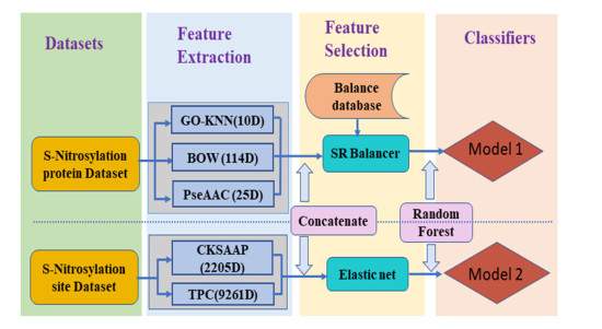
Protein S-nitrosylation is one of the most important post-translational modifications, a well-grounded understanding of S-nitrosylation is very significant since it plays a key role in a variety of biological processes. For an uncharacterized protein sequence, it is a very meaningful problem for both basic research and drug development when we can firstly identify whether it is a S-nitrosylation protein or not, and then predict the specific S-nitrosylation site(s). This work has proposed two models for identifying S-nitrosylation protein and its PTM sites. Firstly, three kinds of features are extracted from protein sequence: KNN scoring of functional domain annotation, PseAAC and bag-of-words based on the physical and chemical properties of amino acids. Secondly, the synthetic minority oversampling technique is used to balance the data sets, and some state-of-the-art classifiers and feature fusion strategies are performed on the balanced data sets. In the five-fold cross-validation for predicting S-nitrosylation proteins, the results of Accuracy (ACC), Matthew's correlation coefficient (MCC) and area under ROC curve (AUC) are 81.84%, 0.5178, 0.8635, respectively. Finally, a model for predicting S-nitrosylation sites has been constructed on the basis of tripeptide composition (TPC) and the composition of $k$-spaced amino acid pairs (CKSAAP). To eliminate redundant information and improve work efficiency, elastic nets are employed for feature selection. The five-fold cross-validation tests have indicated the promising success rates of the proposed model. For the convenience of related researchers, the web-server named "RF-SNOPS" has been established at http://www.jci-bioinfo.cn/RF-SNOPS
- S-nitrosylation,
- random forest,
- post-translational modification,
- multiple features,
- identification
Citation: Wang-Ren Qiu, Qian-Kun Wang, Meng-Yue Guan, Jian-Hua Jia, Xuan Xiao. Predicting S-nitrosylation proteins and sites by fusing multiple features[J]. Mathematical Biosciences and Engineering, 2021, 18(6): 9132-9147. doi: 10.3934/mbe.2021450

Related Papers:

Abstract

http://www.jci-bioinfo.cn/RF-SNOPS]]>

References

[1]	I. Gusarov, E. Nudler, Protein S-nitrosylation: enzymatically controlled, but intrinsically unstable, post-translational modification, Mol. Cell, 69 (2018), 351-353. doi: 10.1016/j.molcel.2018.01.022
[2]	W. Deng, Y. Wang, L. Ma, Y. Zhang, S. Ullah, Y. Xue, Computational prediction of methylation types of covalently modified lysine and arginine residues in proteins, Briefings Bioinf., 18 (2016), 647-658.
[3]	L. Kiemer, J. D. Bendtsen, N. Blom, NetAcet: prediction of N-terminal acetylation sites, Bioinformatics, 21 (2005), 1269-1270. doi: 10.1093/bioinformatics/bti130
[4]	Y. D. Khan, N. Rasool, W. Hussain, S. A. Khan, K. C. Chou, iPhosT-PseAAC: identify phosphothreonine sites by incorporating sequence statistical moments into PseAAC, Anal. Biochem., 550 (2018), 109-116. doi: 10.1016/j.ab.2018.04.021
[5]	M. M. Hasan, B. Manavalan, M. S. Khatun, H. Kurata, Prediction of S-nitrosylation sites by integrating support vector machines and Random Forest, Mol. Omics, 15 (2019), 451-458. doi: 10.1039/C9MO00098D
[6]	V. Fernando, X. Zheng, Y. Walia, V. Sharma, J. Letson, S. Furuta, S-Nitrosylation: an emerging paradigm of redox signaling, Antioxid. (Basel), 8 (2019), 404. doi: 10.3390/antiox8090404
[7]	H. Hayashi, D. T. Hess, R. Zhang, K. Sugi, H. Gao, B. L. Tan, et al., S-nitrosylation of β-arrestins biases receptor signaling and confers ligand independence, Mol. Cell, 70 (2018), 473-487. doi: 10.1016/j.molcel.2018.03.034
[8]	S. Rizza, S. Cardaci, C. Montagna, G. Di Giacomo, D. De Zio, M. Bordi, et al., S-nitrosylation drives cell senescence and aging in mammals by controlling mitochondrial dynamics and mitophagy, Proc. Natl. Acad. Sci., 115 (2018), 3388-3397.
[9]	F. Li, P. Sonveaux, Z. N. Rabbani, S. Liu, B. Yan, Q. Huang, et al., Regulation of HIF-1α stability through S-nitrosylation, Mol. Cell, 26 (2017), 63-74.
[10]	Z. Wang, Protein S-nitrosylation and cancer, Cancer Lett., 320 (2012), 123-129. doi: 10.1016/j.canlet.2012.03.009
[11]	T. S. Wijasa, M. Sylvester, N. Brocke-Ahmadinejad, S. Schwartz, F. Santarelli, V. Gieselmann, et al., Quantitative proteomics of synaptosome S-nitrosylation in Alzheimer's disease, J. Neurochem., 152 (2020), 710-726.
[12]	M. Piroddi, A. Palmese, F. Pilolli, A. Amoresano, P. Pucci, C. Ronco, F. Galli, Plasma nitroproteome of kidney disease patients, Amino Acids, 40 (2011), 653-667. doi: 10.1007/s00726-010-0693-1
[13]	A. Nott, P. M. Watson, J. D. Robinson, L. Crepaldi, A. Riccio, S-nitrosylation of histone deacetylase 2 induces chromatin remodelling in neurons, Nature, 455 (2008), 411-415. doi: 10.1038/nature07238
[14]	G. Huang, J. Li, C. Zhao, Computational prediction and analysis of associations between small molecules and binding-associated S-nitrosylation sites, Molecules, 23 (2018), 954. doi: 10.3390/molecules23040954
[15]	J. R. Burgoyne, P. Eaton, A rapid approach for the detection, quantification, and discovery of novel sulfenic acid or S-nitrosothiol modified proteins using a biotin-switch method, Methods Enzymol., 473 (2010), 281-303.
[16]	G. Hao, B. Derakhshan, L. Shi, F. Campagne, S. S. Gross, SNOSID, a proteomic method for identification of cysteine S-nitrosylation sites in complex protein mixtures, Proc. Natl. Acad. Sci. U. S. A., 103 (2006), 1012-1017.
[17]	W. R. Qiu, B. Q. Sun, X. Xiao, D. Xu, K. C. Chou, iPhos-PseEvo: identifying human phosphorylated proteins by incorporating evolutionary information into general PseAAC via grey system theory, Mol. Inf., 36 (2017), 1600010. doi: 10.1002/minf.201600010
[18]	W. R. Qiu, A. Xu, Z. C. Xu, C. H. Zhang, X. Xiao, Identifying acetylation protein by fusing its PseAAC and functional domain annotation, Front. Bioeng. Biotechnol., 7 (2019), 311. doi: 10.3389/fbioe.2019.00311
[19]	Y. Xue, Z. Liu, X. Gao, C. Jin, L. Wen, X. Yao, J. Ren, GPS-SNO: computational prediction of protein S-nitrosylation sites with a modified GPS algorithm, PLoS One, 5 (2010), e11290. doi: 10.1371/journal.pone.0011290
[20]	T. Y. Lee, Y. J. Chen, T. C. Lu, H. D. Huang, Y. J. Chen, SNOSite: exploiting maximal dependence decomposition to identify cysteine S-nitrosylation with substrate site specificity, PLoS One, 6 (2011), e21849. doi: 10.1371/journal.pone.0021849
[21]	Y. Xu, J. Ding, L. Y. Wu, K. C. Chou, iSNO-PseAAC: predict cysteine S-nitrosylation sites in proteins by incorporating position specific amino acid propensity into pseudo amino acid composition, PLoS One, 8 (2010), e55844.
[22]	A. Siraj, T. Chantsalnyam, H. Tayara, K. T. Chong, RecSNO: prediction of protein S-nitrosylation sites using a recurrent neural network, IEEE Access, 9 (2021), 6674-6682. doi: 10.1109/ACCESS.2021.3096125
[23]	X. Cheng, X. Xiao, K. C. Chou, pLoc_bal-mGneg: predict subcellular localization of gram-negative bacterial proteins by quasi-balancing training dataset and general PseAAC, J. Theor. Biol., 458 (2018), 92-102. doi: 10.1016/j.jtbi.2018.09.005
[24]	K. C. Chou, Some remarks on protein attribute prediction and pseudo amino acid composition, J. Theor. Biol., 273 (2011), 236-247. doi: 10.1016/j.jtbi.2010.12.024
[25]	Y. Z. Chen, Y. R. Tang, Z. Y. Sheng, Z. Zhang, Prediction of mucin-type O-glycosylation sites in mammalian proteins using the composition of k-spaced amino acid pairs, BMC Bioinf., 9 (2008), 101. doi: 10.1186/1471-2105-9-101
[26]	F. N. Auliah, A. N. Nilamyani, W. Shoombuatong, M. A. Alam, M. M. Hasan, H. Kurata, PUP-fuse: prediction of protein pupylation sites by integrating multiple sequence representations, Int. J. Mol. Sci., 22 (2021), 2120. doi: 10.3390/ijms22042120
[27]	Y. Liu, Z. Yu, C. Chen, Y. Han, B. Yu, Prediction of protein crotonylation sites through LightGBM classifier based on SMOTE and elastic net, Anal. Biochem., 609 (2020), 113903. doi: 10.1016/j.ab.2020.113903
[28]	Y. Xie, X. Luo, Y. Li, L. Chen, W. Ma, J. Huang, et al., DeepNitro: prediction of protein nitration and nitrosylation sites by deep learning, Genomics, Proteomics Bioinf., 16 (2018), 294-306. doi: 10.1016/j.gpb.2018.04.007
[29]	W. Qiu, Z. Lv, Y. Hong, J. Jia, X. Xiao, BOW-GBDT: a GBDT classifier combining with artificial neural network for identifying GPCR-drug interaction based on wordbook learning from sequences, Front. Cell Dev. Biol., 8 (2021), 623858. doi: 10.3389/fcell.2020.623858
[30]	S. Kawashima, M. Kanehisa, AAindex: amino acid index database, Nucleic Acids Res., 28 (2000), 374. doi: 10.1093/nar/28.1.374
[31]	N. V. Chawla, K. W. Bowyer, L. O. Hall, W. P. Kegelmeyer, SMOTE: synthetic minority over-sampling technique, J. Artif. Intell. Res., 16 (2002), 321-357. doi: 10.1613/jair.953
[32]	M. J. Kim, D. K. Kang, H. B. Kim, Geometric mean based boosting algorithm with over-sampling to resolve data imbalance problem for bankruptcy prediction, Expert Syst. Appl., 42 (2015), 1074-1082. doi: 10.1016/j.eswa.2014.08.025
[33]	S. Yan, W. Qian, Y. Guan, B. Zheng, Improving lung cancer prognosis assessment by incorporating synthetic minority oversampling technique and score fusion method, Med. Phys., 43 (2016), 2694-2703. doi: 10.1118/1.4948499
[34]	N. Habib, M. M. Hasan, M. M. Reza, M. M. Rahman, Ensemble of CheXNet and VGG-19 feature extractor with Random Forest classifier for pediatric pneumonia detection, SN Comput. Sci., 1 (2020), 359. doi: 10.1007/s42979-020-00373-y
[35]	K. Ghosh, A. Sarkar, A. Banerjee, S. Chatterjee. Performance improvement of convolutional neural network using random under sampling, in Advances in Smart Communication Technology and Information Processing, Springer, (2021), 207-217.
[36]	S. Hua, Z. Sun, Support vector machine approach for protein subcellular localization prediction, Bioinformatics, 17 (2001), 721-728. doi: 10.1093/bioinformatics/17.8.721
[37]	H. Bian, M. Guo, J. Wang, Recognition of mitochondrial proteins in plasmodium based on the tripeptide composition, Front. Cell Dev. Biol., 8 (2020), 578901. doi: 10.3389/fcell.2020.578901
[38]	H. Zou, T. Hastie, Regularization and variable selection via the elastic net, J. R. Stat. Soc. Ser. B (Stat. Methodol.), 67 (2005), 301-320. doi: 10.1111/j.1467-9868.2005.00503.x
[39]	G. Chen, M. Cao, J. Yu, X. Guo, S. Shi, Prediction and functional analysis of prokaryote lysine acetylation site by incorporating six types of features into Chou's general PseAAC, J. Theor. Biol., 461 (2019), 92-101. doi: 10.1016/j.jtbi.2018.10.047
[40]	W. R. Qiu, B. Q. Sun, X. Xiao, Z. C. Xu, J. H. Jia, K. C. Chou, iKcr-PseEns: identify lysine crotonylation sites in histone proteins with pseudo components and ensemble classifier, Genomics, 110 (2018), 239-246. doi: 10.1016/j.ygeno.2017.10.008
[41]	L. Breiman, Random Forests. Mach. Learn., 45 (2001), 5-32. doi: 10.1023/A:1010933404324
[42]	H. Talebi, L. J. M. Peeters, A. Otto, R. Tolosana-Delgado, A truly spatial Random Forests algorithm for geoscience data analysis and modelling, Math. Geosci., 2021.
[43]	Z. Qiu, Q. Liu, Protein-protein interaction site prediction using random forest proximity distance, J. Bioinf. Comput. Biol., 19 (2021), 2050042. doi: 10.1142/S0219720020500420
[44]	S. Cabras, M. E. Castellanos, E. Staffetti, A Random Forest application to contact-state classification for robot programming by human demonstration, Appl. Stochastic Models Bus. Ind., 32 (2016), 209-227. doi: 10.1002/asmb.2145
[45]	N. Friedman, D. Geiger, M. Goldszmidt, Bayesian network classifiers, Mach. Learn., 29 (1997), 131-163. doi: 10.1023/A:1007465528199
[46]	R. Queiroz, T. Berger, K. Czarnecki, Towards predicting feature defects in software product lines, in Proceedings of the 7th International Workshop on Feature-Oriented Software Development, Amsterdam, Netherlands, Association for Computing Machinery, (2016), 58-62.
[47]	H. Bohra, A. Arora, P. Gaikwad, R. Bhand, M. R. Patil, Health prediction and medical diagnosis using Naive Bayes, Ijarcce, 6 (2017), 32-35.
[48]	M. S. Ahmed, M. Shahjaman, E. Kabir, M. Kamruzzaman, Prediction of protein acetylation sites using kernel Naive Bayes classifier based on protein sequences profiling, Bioinformation, 14 (2018), 213-218. doi: 10.6026/97320630014213
[49]	F. Nigsch, A. Bender, B. van Buuren, J. Tissen, E. Nigsch, J. B. Mitchell, Melting point prediction employing K-Nearest Neighbor algorithms and genetic parameter optimization, J. Chem. Inf. Model., 46 (2006), 2412-2422. doi: 10.1021/ci060149f
[50]	A. Wirdiani, P. Hridayami, A. Widiari, K. Rismawan, P. Candradinata, I. Jayantha, Face identification based on K-Nearest Neighbor, Sci. J. Inf., 6 (2019), 150-159.
[51]	O. Borgohain, M. Dasgupta, P. Kumar, G. Talukdar, Performance analysis of nearest neighbor, K-Nearest Neighbor and weighted K-Nearest Neighbor for the cassification of Alzheimer disease, in Soft Computing Techniques and Applications, S. Borah, R. Pradhan, N. Dey, P. Gupta, Ed., Springer, Singapore, (2021), 295-304.
[52]	S. Huang, M. Huang, Y. Lyu, A novel approach for sand liquefaction prediction via local mean-based pseudo nearest neighbor algorithm and its engineering application, Adv. Eng. Inf., 41 (2019), 100918. doi: 10.1016/j.aei.2019.04.008
[53]	T. Chen, C. Guestrin, XGBoost: a scalable tree boosting system, in Proceedings of the 22nd ACM SIGKDD International Conference on Knowledge Discovery and Data Mining, San Francisco, California, USA, Association for Computing Machinery, (2016), 785-794.
[54]	I. Babajide Mustapha, F. Saeed, Bioactive molecule prediction using extreme gradient boosting, Molecules, 21 (2016), 983. doi: 10.3390/molecules21080983
[55]	J. H. Friedman, Greedy function approximation: a gradient boosting machine, Ann. Stat., 29 (2001), 1189-1232. doi: 10.1214/aos/1013203450

Reader Comments

Your name:*

Email:*
© 2021 the Author(s), licensee AIMS Press. This is an open access article distributed under the terms of the Creative Commons Attribution License (http://creativecommons.org/licenses/by/4.0)