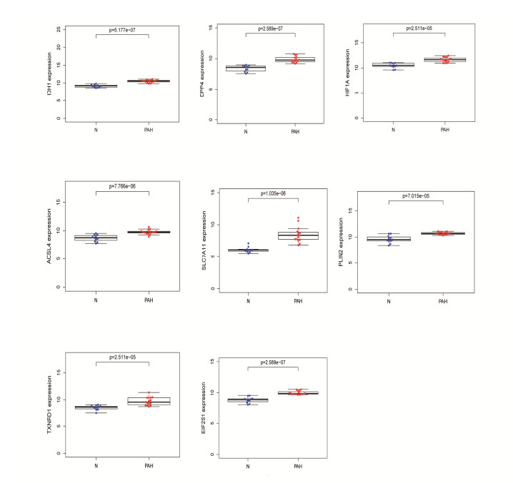
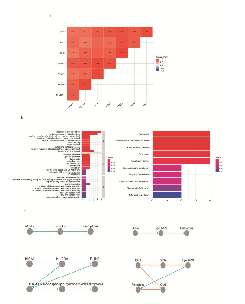
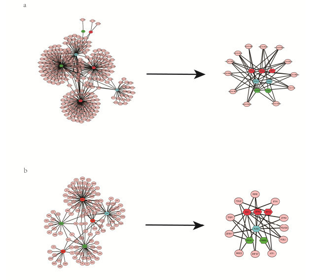
Pulmonary arterial hypertension (PAH) is a life-threatening illness and ferroptosis is an iron-dependent form of regulated cell death, driven by the accumulation of lipid peroxides to levels that are sufficient to trigger cell death. However, only few studies have examined PAH-associated ferroptosis. In the present study, lung samples mRNA expression profiles (derived from 15 patients with PAH and 11 normal controls) were downloaded from a public database, and 514 differentially expressed genes (DEGs) were identified using the Wilcoxon rank-sum test and weighted gene correlation network analyses. These DEGs were screened for ferroptosis-associated genes using the FerrDb database: eight ferroptosis-associated genes were identified. Finally, the construction of gene-microRNA (miRNA) and gene-transcription factor (TF) networks, in conjunction with gene ontology and biological pathway enrichment analysis, were used to inform hypotheses regarding the molecular mechanisms underlying PAH-associated ferroptosis. Ferroptosis-associated genes were largely involved in oxidative stress responses and could be regulated by several identified miRNAs and TFs. This suggests the existence of modulatable pathways that are potentially involved in PAH-associated ferroptosis. Our findings provide novel directions for targeted therapy of PAH in regard to ferroptosis. These findings may ultimately help improve the therapeutic outcomes of PAH.
Citation: Fan Zhang, Hongtao Liu. Identification of ferroptosis-associated genes exhibiting altered expression in pulmonary arterial hypertension[J]. Mathematical Biosciences and Engineering, 2021, 18(6): 7619-7630. doi: 10.3934/mbe.2021377
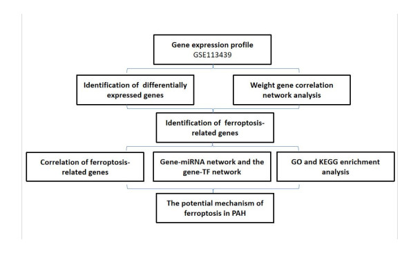
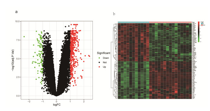
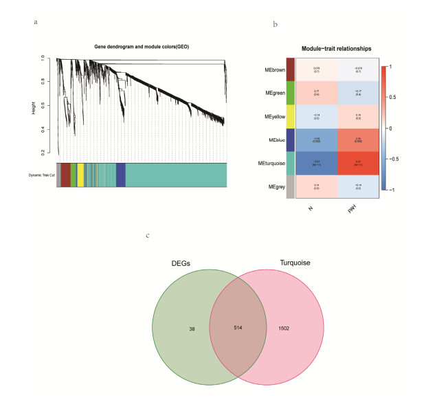
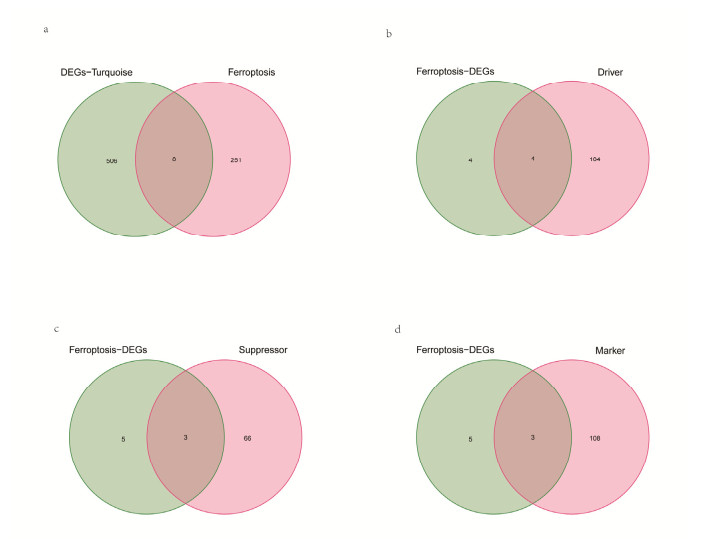
Pulmonary arterial hypertension (PAH) is a life-threatening illness and ferroptosis is an iron-dependent form of regulated cell death, driven by the accumulation of lipid peroxides to levels that are sufficient to trigger cell death. However, only few studies have examined PAH-associated ferroptosis. In the present study, lung samples mRNA expression profiles (derived from 15 patients with PAH and 11 normal controls) were downloaded from a public database, and 514 differentially expressed genes (DEGs) were identified using the Wilcoxon rank-sum test and weighted gene correlation network analyses. These DEGs were screened for ferroptosis-associated genes using the FerrDb database: eight ferroptosis-associated genes were identified. Finally, the construction of gene-microRNA (miRNA) and gene-transcription factor (TF) networks, in conjunction with gene ontology and biological pathway enrichment analysis, were used to inform hypotheses regarding the molecular mechanisms underlying PAH-associated ferroptosis. Ferroptosis-associated genes were largely involved in oxidative stress responses and could be regulated by several identified miRNAs and TFs. This suggests the existence of modulatable pathways that are potentially involved in PAH-associated ferroptosis. Our findings provide novel directions for targeted therapy of PAH in regard to ferroptosis. These findings may ultimately help improve the therapeutic outcomes of PAH.

| [1] |
G. Mansueto, M. D. Napoli, C.P. Campobasso, M. Slevin, Pulmonary arterial hypertension (PAH) from autopsy study: T-cells, B-cells and mastocytes detection as morphological evidence of immunologically mediated pathogenesis, Pathol. Res. Pract., 225 (2021), 153552. doi: 10.1016/j.prp.2021.153552

|
| [2] |
S. Gräf, M. Haimel, M. Bleda, C. Hadinnapola, L. Southgate, W. Li, et al., Identification of rare sequence variation underlying heritable pulmonary arterial hypertension, Nat. Commun., 9 (2018), 1416. doi: 10.1038/s41467-018-03672-4
|
| [3] |
T. Hiraide, M. Kataoka, H. Suzuki, Y. Aimi, T. Chiba, K. Kanekura, et al., SOX17 Mutations in Japanese Patients with Pulmonary Arterial Hypertension, Am. J. Respir. Crit. Care Med., 198 (2018), 1231-1233. doi: 10.1164/rccm.201804-0766LE
|
| [4] |
S. J. Dixon, K. M. Lemberg, M. R. Lamprecht, R. Skouta, E. M. Zaitsev, C. E. Gleason, et al., Ferroptosis: an iron-dependent form of nonapoptotic cell death, Cell, 149 (2012), 1060-1072. doi: 10.1016/j.cell.2012.03.042
|
| [5] |
Y. C. Li, Y. M. Cao, J. Xiao, J. W. Shang, Q. Tan, F. Ping, et al., Inhibitor of apoptosis-stimulating protein of p53 inhibits ferroptosis and alleviates intestinal ischemia/reperfusion-induced acute lung injury, Cell Death Differ., 27 (2020), 2635-2650. doi: 10.1038/s41418-020-0528-x
|
| [6] |
X. Li, L. J. Duan, S. J. Yuan, X. B. Zhuang, T. K. Qiao, J. He, Ferroptosis inhibitor alleviates Radiation-induced lung fibrosis (RILF) via down-regulation of TGF-β1, J. Inflamm. (Lond)., 16 (2019), 11. doi: 10.1186/s12950-019-0216-0
|
| [7] |
M. Mura, M. J. Cecchini, M. Joseph, J. T. Granton, Osteopontin lung gene expression is a marker of disease severity in pulmonary arterial hypertension, Respirology, 24 (2019), 1104-1110. doi: 10.1111/resp.13557
|
| [8] | T. Barrett, S. E. Wilhite, P. Ledoux, C. Evangelista, I. F. Kim, M. Tomashevsky, et al., NCBI GEO: archive for functional genomics data sets--update, Nucleic Acids Res., 41 (2013), D991-D995. |
| [9] |
H. Jalal, P. Pechlivanoglou, E. Krijkamp, F. Alarid-Escudero, E. Enns, M. G. M. Hunink, An overview of R in health decision sciences, Med. Decis. Making, 37 (2017), 735-746. doi: 10.1177/0272989X16686559
|
| [10] |
M. E. Ritchie, B. Phipson, D. Wu, Y. F. Hu, C. W. Law, W. Shi, et al., Limma powers differential expression analyses for RNA-sequencing and microarray studies, Nucleic Acids Res., 43 (2015), e47. doi: 10.1093/nar/gkv007
|
| [11] | K. Ito, D. Murphy, Application of ggplot2 to Pharmacometric Graphics, CPT Pharmacometrics Syst. Pharmacol., 2 (2013), 1-16. |
| [12] | R. Kolde, Pheatmap: pretty heatmaps, R package version, 1.0.8., 2015. Available from: https://CRAN.R-project.org/package=pheatmap. |
| [13] |
P. Langfelder, S. Horvath, WGCNA: an R package for weighted correlation network analysis, BMC Bioinf., 9 (2008), 559. doi: 10.1186/1471-2105-9-559
|
| [14] |
H. B. Chen, P.C. Boutros, VennDiagram: a package for the generation of highly-customizable Venn and Euler diagrams in R, BMC Bioinf., 12 (2011), 35. doi: 10.1186/1471-2105-12-35
|
| [15] | N. Zhou, J. K. Bao, FerrDb: a manually curated resource for regulators and markers of ferroptosis and ferroptosis-disease associations, Database, 2020 (2020). |
| [16] | A. Eklund, Beeswarm: the bee swarm plot, an alternative to stripchart, R package version, 0.2.3., 2016. Available from: https://cran.r-project.org/package=beeswarm. |
| [17] | H. A. Kassambara, Ggpubr: "ggplot2" based punlication ready plots, R package version, 1.0.7., 2018. Available from: https://cran.r-project.org/install.packages ("ggpubr"). |
| [18] |
G. C. Yu, L. G. Wang, Y. Y. Han, Q. Y. He, clusterProfiler: an R package for comparing biological themes among gene clusters, Omics: J. Integr. Biol., 16 (2012), 284-287. doi: 10.1089/omi.2011.0118
|
| [19] | B. Nota, Gogadget: An R package for interpretation and visualization of GO enrichment results, Mol. Inf., 36 (2017), 5-6. |
| [20] |
M. Kanehisa, M. Furumichi, M. Tanabe, Y. Sato, K. Morishima, KEGG: new perspectives on genomes, pathways, diseases and drugs, Nucleic Acids Res., 45 (2017), D353-D361. doi: 10.1093/nar/gkw1092
|
| [21] |
S. D. Hsu, F. M. Lin, W. Y. Wu, C. Liang, W. C. Huang, W. L. Chan, et al., miRTarBase: a database curates experimentally validated microRNA-target interactions, Nucleic Acids Res., 39 (2011), D163-D169. doi: 10.1093/nar/gkq1107
|
| [22] |
J. R. Ecker, W. A. Bickmore, I. Barroso, J. K. Pritchard, Y. Gilad, E. Segal, Genomics: ENCODE explained, Nature, 489 (2012), 52-55. doi: 10.1038/489052a
|
| [23] |
J. Reimand, R. Isserlin, V. Voisin, M. Kucera, C. Tannus-Lopes, A. Rostamianfar, et al., Pathway enrichment analysis and visualization of omics data using g: Profiler, GSEA, Cytoscape and EnrichmentMap, Nat. Protoc., 14 (2019), 482-517. doi: 10.1038/s41596-018-0103-9
|
| [24] |
L. Hecker, Mechanisms and consequences of oxidative stress in lung disease: therapeutic implications for an aging populace, Am. J. Physiol. Lung Cell Mol. Physiol., 314 (2018), L642-L653. doi: 10.1152/ajplung.00275.2017
|
| [25] |
P. A. Kirkham, P. J. Barnes, Oxidative stress in COPD, Chest, 144 (2013), 266-273. doi: 10.1378/chest.12-2664
|
| [26] |
E. A. Zemskov, Q. Lu, W. Ornatowski, C. N. Klinger, A. A. Desai, E. Maltepe, et al., Biomechanical forces and oxidative stress: implications for pulmonary vascular disease, Antioxid. Redox Signaling, 31 (2019), 819-842. doi: 10.1089/ars.2018.7720
|
| [27] | S. Aggarwal, C. M. Gross, S. Sharma, J. R. Fineman, S. M. Black, Reactive oxygen species in pulmonary vascular remodeling, Compr. Physiol., 3 (2013), 1011-1034. |
| [28] |
W. S. Yang, B. R. Stockwell, Ferroptosis: death by lipid peroxidation, Trends Cell Biol., 26 (2016), 165-176. doi: 10.1016/j.tcb.2015.10.014
|
| [29] |
L. B. Frankel, A. H. Lund, MicroRNA regulation of autophagy, Carcinogenesis, 33 (2012), 2018-2025. doi: 10.1093/carcin/bgs266
|
| [30] |
D. P. Bartel, MicroRNAs: genomics, biogenesis, mechanism, and function, Cell, 116 (2004), 281-297. doi: 10.1016/S0092-8674(04)00045-5
|
| [31] |
M. Y. Luo, L. F. Wu, K. X. Zhang, H. Wang, T. Zhang, L. Gutierrez, et al., miR-137 regulates ferroptosis by targeting glutamine transporter SLC1A5 in melanoma, Cell Death Differ., 25 (2018), 1457-1472. doi: 10.1038/s41418-017-0053-8
|
| [32] |
X. L. Lai, A. Stigliani, G. Vachon, C. Carles, C. Smaczniak, C. Zubieta, et al., Building transcription factor binding site models to understand gene regulation in plants, Mol. Plant., 12 (2019), 743-763. doi: 10.1016/j.molp.2018.10.010
|
| [33] |
J. M. Vaquerizas, S. K. Kummerfeld, S. A. Teichmann, N. M. Luscombe, A census of human transcription factors: function, expression and evolution, Nat. Rev. Genet., 10 (2009), 252-263. doi: 10.1038/nrg2538
|
 mbe-18-06-377-supplementary.xls mbe-18-06-377-supplementary.xls |
 |
Figures(7)

Fan Zhang, Hongtao Liu. Identification of ferroptosis-associated genes exhibiting altered expression in pulmonary arterial hypertension[J]. Mathematical Biosciences and Engineering, 2021, 18(6): 7619-7630. doi: 10.3934/mbe.2021377


 DownLoad: