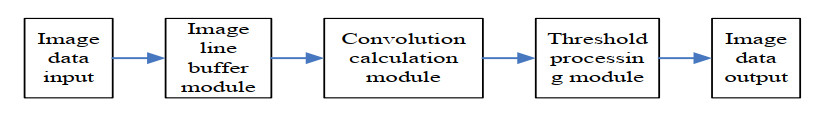
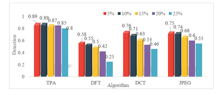
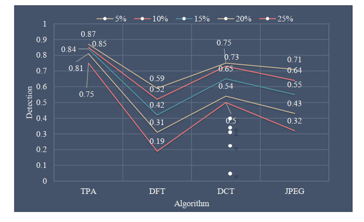
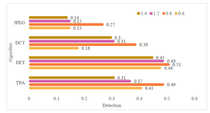
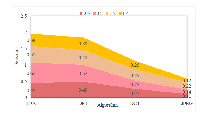
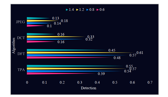
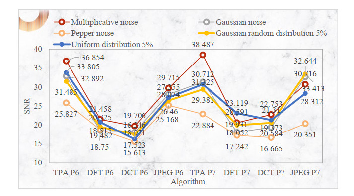
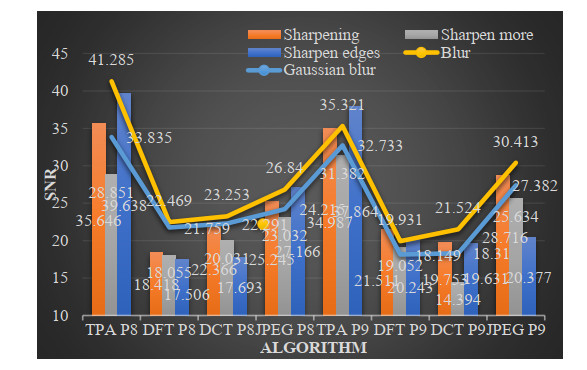
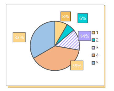
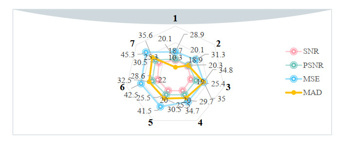
With the rapid development of computer technology and network communication technology, copyright protection caused by widely spread digital media has become the focus of attention in various fields. For digital media watermarking technology research emerge in endlessly, but the results are not ideal. In order to better realize the copyright identification and protection, based on the embedded intelligent edge computing detection technology, this paper studies the zero watermark copyright protection algorithm of digital media. Firstly, this paper designs an embedded intelligent edge detection module based on Sobel operator, including image line buffer module, convolution calculation module and threshold processing module. Then, based on the embedded intelligent edge detection module, the Arnold transform of image scrambling technology is used to preprocess the watermark, and finally a zero watermark copyright protection algorithm is constructed. At the same time, the robustness of the proposed algorithm is tested. The image is subjected to different proportion of clipping and scaling attacks, different types of noise, sharpening and blur attacks, and the detection rate and signal-to-noise ratio of each algorithm are calculated respectively. The performance of the watermark image processed by this algorithm is evaluated subjectively and objectively. Experimental data show that the detection rate of our algorithm is the highest, which is 0.89. In scaling attack, the performance of our algorithm is slightly lower than that of Fourier transform domain algorithm, but it is better than the other two algorithms. The Signal to Noise Ratio of the algorithm is 36.854% in P6 multiplicative noise attack, 39.638% in P8 sharpening edge attack and 41.285% in fuzzy attack. This shows that the algorithm is robust to conventional attacks. The subjective evaluation of 33% and 39% of the images is 5 and 4. The mean values of signal to noise ratio, peak signal to noise ratio, mean square error and mean absolute difference are 20.56, 25.13, 37.03 and 27.64, respectively. This shows that the watermark image processed by this algorithm has high quality. Therefore, the digital media zero watermark copyright protection algorithm based on embedded intelligent edge computing detection is more robust, and its watermark invisibility is also very superior, which is worth promoting.
Citation: Hongyan Xu. Digital media zero watermark copyright protection algorithm based on embedded intelligent edge computing detection[J]. Mathematical Biosciences and Engineering, 2021, 18(5): 6771-6789. doi: 10.3934/mbe.2021336
With the rapid development of computer technology and network communication technology, copyright protection caused by widely spread digital media has become the focus of attention in various fields. For digital media watermarking technology research emerge in endlessly, but the results are not ideal. In order to better realize the copyright identification and protection, based on the embedded intelligent edge computing detection technology, this paper studies the zero watermark copyright protection algorithm of digital media. Firstly, this paper designs an embedded intelligent edge detection module based on Sobel operator, including image line buffer module, convolution calculation module and threshold processing module. Then, based on the embedded intelligent edge detection module, the Arnold transform of image scrambling technology is used to preprocess the watermark, and finally a zero watermark copyright protection algorithm is constructed. At the same time, the robustness of the proposed algorithm is tested. The image is subjected to different proportion of clipping and scaling attacks, different types of noise, sharpening and blur attacks, and the detection rate and signal-to-noise ratio of each algorithm are calculated respectively. The performance of the watermark image processed by this algorithm is evaluated subjectively and objectively. Experimental data show that the detection rate of our algorithm is the highest, which is 0.89. In scaling attack, the performance of our algorithm is slightly lower than that of Fourier transform domain algorithm, but it is better than the other two algorithms. The Signal to Noise Ratio of the algorithm is 36.854% in P6 multiplicative noise attack, 39.638% in P8 sharpening edge attack and 41.285% in fuzzy attack. This shows that the algorithm is robust to conventional attacks. The subjective evaluation of 33% and 39% of the images is 5 and 4. The mean values of signal to noise ratio, peak signal to noise ratio, mean square error and mean absolute difference are 20.56, 25.13, 37.03 and 27.64, respectively. This shows that the watermark image processed by this algorithm has high quality. Therefore, the digital media zero watermark copyright protection algorithm based on embedded intelligent edge computing detection is more robust, and its watermark invisibility is also very superior, which is worth promoting.

| [1] |
Q. Zhu, Digital watermarking technology based on relational database, J. Interdiscip. Math., 21 (2018), 1211-1215. doi: 10.1080/09720502.2018.1495226

|
| [2] |
Nasr addin Ahmed Salem Al-maweri, R. Ali, W. A. W. Adnan, A. R. Ramli, S. M. S. Ahmad, State-of-the-Art in Techniques of Text Digital Watermarking: Challenges and Limitations, J. Comput. Sci., 12 (2016), 62-80. doi: 10.3844/jcssp.2016.62.80
|
| [3] |
C. Wang, X. Wang, Z. Xia, C. Zhang, Ternary radial harmonic Fourier moments based robust stereo image zero-watermarking algorithm, Inf. Sci., 470 (2019), 109-120. doi: 10.1016/j.ins.2018.08.028
|
| [4] |
Z. Xia, X. Wang, B. Han, Q. Li, T. Zhao, Color image triple zero-watermarking using decimal-order polar harmonic transforms and chaotic system, Signal Process., 180 (2021), 107864. doi: 10.1016/j.sigpro.2020.107864
|
| [5] |
X. Zhang, Z. Shen, Copyright protection method for 3D model of geological body based on digital watermarking technology, J. Visual Commun. Image Representation, 59 (2019), 334-346. doi: 10.1016/j.jvcir.2018.12.013
|
| [6] | X. H. Wang, D. H. Wei, X. X. Liu, X. C. Ma, Digital watermarking technique of color image based on color QR code, J. Optoelectron. Laser, 27 (2016), 1094-1100. |
| [7] |
X. Yang, W. Dai, G. Tang, L. Min, Deriving Ephemeral Gullies from VHR Image in Loess Hilly Areas through Directional Edge Detection, ISPRS Int. J. Geo Inf., 6 (2017), 371-371. doi: 10.3390/ijgi6110371
|
| [8] | H. Dadgostar, F. Afsari. Image steganography based on interval-valued intuitionistic fuzzy edge detection and modified LSB, Inf. Secur. Tech. Rep., 30 (2016), 94-104. |
| [9] | R. Thankachan, R. Sethunadh, P. Ameer. Edge Detection in Polarimetric SAR Image based on Bandelet Transform, Int. J. Comput. Appl., 181 (2019), 33-38. |
| [10] |
P. M. Shakeel, S. Baskar, R. Sampath, M. M. Jaber, Echocardiography image segmentation using feed forward artificial neural network (FFANN) with fuzzy multi-scale edge detection (FMED), Int. J. Signal Imaging Syst. Eng., 11 (2019), 270-270. doi: 10.1504/IJSISE.2019.100651
|
| [11] | J. Jumanto. An Enhanced LSB-Image Steganography Using the Hybrid Canny-Sobel Edge Detection, Cybernetics Inf. Technol., 18 (2018), 74-88. |
| [12] | D. Nagarajan, M. Lathamaheswari, R. Sujatha, J. Kavikumar, Edge Detection on DICOM Image using Triangular Norms in Type-2 Fuzzy, Int. J. Adv. Comput. Sci. Appl., 9 (2018), 462-275. |
| [13] | Y. Zhang, X. L. Ma. Research on image digital watermarking optimization algorithm under virtual reality technology, Discrete Contin. Dyn. Syst., 12 (2019), 1427-1440. |
| [14] |
H. Tan, P. Tang, C. Zhang, Digital Watermarking for Color Images Based on Compressive Sensing, Nanoence Nanotechnol. Lett., 9 (2017), 724-729. doi: 10.1166/nnl.2017.2279
|
| [15] |
A. Q. M. Sabri, A. M. Mansoor, U. H. Obaidellah, E. R. M. Faizal, J. L. PC, Metadata hiding for UAV video based on digital watermarking in DWT transform, Multimedia Tools Appl., 76 (2017), 16239-16261. doi: 10.1007/s11042-016-3906-0
|
| [16] | C. L. Song, L. Yang, X. Wang. Secure and Robust Digital Watermarking: A Survey, J. Electron. Sci. Technol., 14 (2016), 57-68. |
| [17] |
Nasr addin Ahmed Salem Al-maweri, R. Ali, W. A. W. Adnan, A. R. Ramli, S. M. S. Ahmad, State-of-the-Art in Techniques of Text Digital Watermarking: Challenges and Limitations, J. Comput. Sci., 12 (2016), 62-80. doi: 10.3844/jcssp.2016.62.80
|
| [18] | Z. Ling, Anti-tampering technology of digital watermarking in dynamic web page images, Agro Food Ind. Hi Tech, 28 (2017), 2195-2199. |
| [19] | Y. Zhang, C. Wang, X. Wang, W. Min, Feature-Based Image Watermarking Algorithm Using SVD and APBT for Copyright Protection, Future Internet, 9 (2017), 1-13. |
| [20] | C. Chongtham, M. S. Khumanthem, Y. J. Chanu, N. Arambam, D. Meitei, P. R. Chanu, et al., A Copyright Protection Scheme for Videos Based on the SIFT, Iran. J. Sci. Technol., Trans. Electr. Eng., 42 (2018), 107-121. |
| [21] |
Z. Xia, X. Wang, X. Li, C. Wang, S. Unar, M. Wang, et al., Efficient copyright protection for three CT images based on quaternion polar harmonic Fourier moments, Signal Process., 164 (2019), 368-379. doi: 10.1016/j.sigpro.2019.06.025
|
| [22] |
X. W. Li, S. T. Kim, Q. H. Wang, Copyright protection for elemental image array by hypercomplex Fourier transform and an adaptive texturized holographic algorithm, Opt. Express, 25 (2017), 17076-17098. doi: 10.1364/OE.25.017076
|
| [23] | R. Mancha, Adaptive Image Watermarking Scheme Using Fuzzy Entropy and GA-ELM Hybridization in DCT Domain for Copyright Protection. J. Signal Process. Syst., 84 (2016), 265-281. |
| [24] | A. Lakshmi Priya, S. Letitia, Copyright Protection for Digital Colour Images Using Dual Watermarking Technique by Applying Improved DWT, DCT and SVD, J. Electr. Electron. Eng., 4 (2016), 120-130. |
| [25] | A. E. Afify, A. Emran, A. Yahya, A Tamper Proofing Text Watermarking Shift Algorithm for Copyright Protection, Arab J. Nuclear Sci. Appl., 52 (2019), 126-133. |
Figures(10) / Tables(4)

Hongyan Xu. Digital media zero watermark copyright protection algorithm based on embedded intelligent edge computing detection[J]. Mathematical Biosciences and Engineering, 2021, 18(5): 6771-6789. doi: 10.3934/mbe.2021336


 DownLoad: