A simple model of cardiac mitochondrial respiration with experimental validation

Bachar Tarraf; Emmanuel Suraniti; Camille Colin; Stéphane Arbault; Philippe Diolez; Michael Leguèbe; Yves Coudière; Bachar Tarraf; Emmanuel Suraniti; Camille Colin; Stéphane Arbault; Philippe Diolez; Michael Leguèbe; Yves Coudière

doi:10.3934/mbe.2021291

Mathematical Biosciences and Engineering

2021, Volume 18, Issue 5: 5758-5789. doi: 10.3934/mbe.2021291

Previous Article Next Article

Research article Special Issues

A simple model of cardiac mitochondrial respiration with experimental validation

1.
Inria Bordeaux-Sud-Ouest, team CARMEN, Talence, France
2.
IHU Liryc, Fondation Bordeaux Université, Pessac, France
3.
Institut de Mathématiques de Bordeaux, UMR CNRS 5251, Talence, France
4.
Université de Bordeaux, Bordeaux, France
5.
ISM, CNRS UMR 5255, Bordeaux, France
6.
INSERM, Centre de Recherche Cardio-Thoracique de Bordeaux, U-1045, Bordeaux, France

Received: 12 February 2021 Accepted: 06 June 2021 Published: 25 June 2021

Cardiac mitochondria are intracellular organelles that play an important role in energy metabolism and cellular calcium regulation. In particular, they influence the excitation-contraction cycle of the heart cell. A large number of mathematical models have been proposed to better understand the mitochondrial dynamics, but they generally show a high level of complexity, and their parameters are very hard to fit to experimental data.

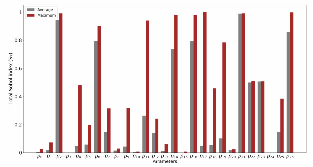
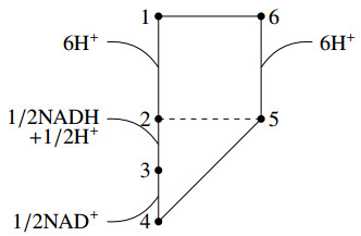
We derived a model based on historical free energy-transduction principles, and results from the literature. We proposed simple expressions that allow to reduce the number of parameters to a minimum with respect to the mitochondrial behavior of interest for us. The resulting model has thirty-two parameters, which are reduced to twenty-three after a global sensitivity analysis of its expressions based on Sobol indices.

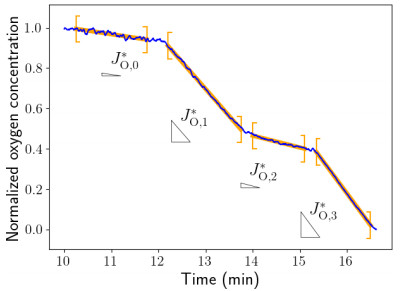
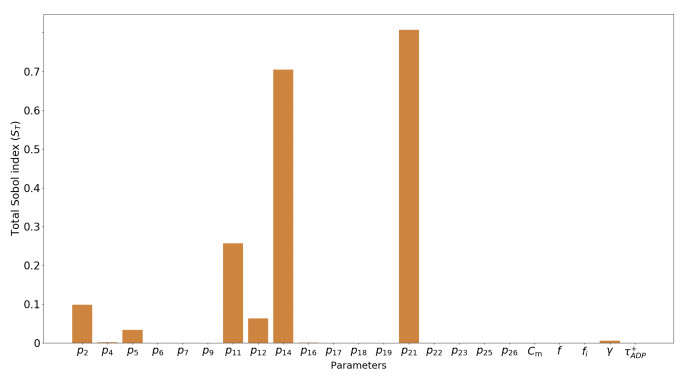
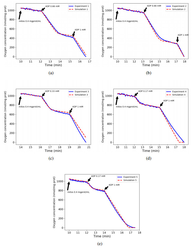
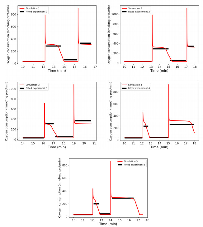
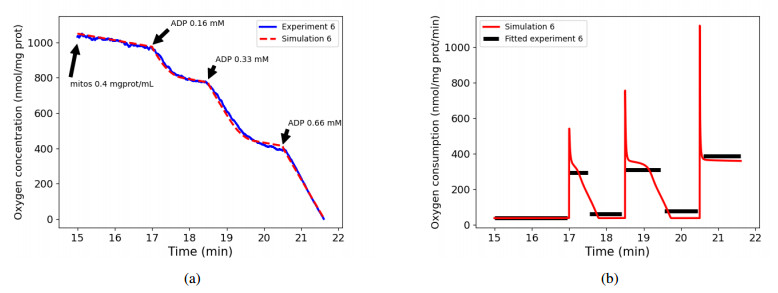
We calibrated our model to experimental data that consists of measurements of mitochondrial respiration rates controlled by external ADP additions. A sensitivity analysis of the respiration rates showed that only seven parameters can be identified using these observations. We calibrated them using a genetic algorithm, with five experimental data sets. At last, we used the calibration results to verify the ability of the model to accurately predict the values of a sixth dataset.

Results show that our model is able to reproduce both respiration rates of mitochondria and transitions between those states, with very low variability of the parameters between each experiment. The same methodology may apply to recover all the parameters of the model, if corresponding experimental data were available.

Keywords:

Citation: Bachar Tarraf, Emmanuel Suraniti, Camille Colin, Stéphane Arbault, Philippe Diolez, Michael Leguèbe, Yves Coudière. A simple model of cardiac mitochondrial respiration with experimental validation[J]. Mathematical Biosciences and Engineering, 2021, 18(5): 5758-5789. doi: 10.3934/mbe.2021291

Related Papers:

[1]	Yue Cao . Blow-up criterion for the 3D viscous polytropic fluids with degenerate viscosities. Electronic Research Archive, 2020, 28(1): 27-46. doi: 10.3934/era.2020003
[2]	Jie Zhang, Gaoli Huang, Fan Wu . Energy equality in the isentropic compressible Navier-Stokes-Maxwell equations. Electronic Research Archive, 2023, 31(10): 6412-6424. doi: 10.3934/era.2023324
[3]	Jianxia He, Qingyan Li . On the global well-posedness and exponential stability of 3D heat conducting incompressible Navier-Stokes equations with temperature-dependent coefficients and vacuum. Electronic Research Archive, 2024, 32(9): 5451-5477. doi: 10.3934/era.2024253
[4]	Yazhou Wang, Yuzhu Wang . Regularity criterion of three dimensional magneto-micropolar fluid equations with fractional dissipation. Electronic Research Archive, 2024, 32(7): 4416-4432. doi: 10.3934/era.2024199
[5]	Guochun Wu, Han Wang, Yinghui Zhang . Optimal time-decay rates of the compressible Navier–Stokes–Poisson system in $\mathbb R^3$ . Electronic Research Archive, 2021, 29(6): 3889-3908. doi: 10.3934/era.2021067
[6]	Jie Qi, Weike Wang . Global solutions to the Cauchy problem of BNSP equations in some classes of large data. Electronic Research Archive, 2024, 32(9): 5496-5541. doi: 10.3934/era.2024255
[7]	Hui Yang, Futao Ma, Wenjie Gao, Yuzhu Han . Blow-up properties of solutions to a class of $p$ -Kirchhoff evolution equations. Electronic Research Archive, 2022, 30(7): 2663-2680. doi: 10.3934/era.2022136
[8]	Yang Cao, Qiuting Zhao . Initial boundary value problem of a class of mixed pseudo-parabolic Kirchhoff equations. Electronic Research Archive, 2021, 29(6): 3833-3851. doi: 10.3934/era.2021064
[9]	José Luis Díaz Palencia, Saeed Ur Rahman, Saman Hanif . Regularity criteria for a two dimensional Erying-Powell fluid flowing in a MHD porous medium. Electronic Research Archive, 2022, 30(11): 3949-3976. doi: 10.3934/era.2022201
[10]	Zhonghua Qiao, Xuguang Yang . A multiple-relaxation-time lattice Boltzmann method with Beam-Warming scheme for a coupled chemotaxis-fluid model. Electronic Research Archive, 2020, 28(3): 1207-1225. doi: 10.3934/era.2020066

Abstract

1. Introduction

We consider the compressible isentropic Navier-Stokes equations with degenerate viscosities in $\mathbb{R}^3$ , which gives the conservation laws of mass and momentum of fluids. This model comes from the Boltzmann equations through the Chapman-Enskog expansion to the second order, and the viscosities depend on the density $\rho\geq 0$ by the laws of Boyle and Gay-Lussac for ideal gas. This system can be written as

$\begin{equation} \left\{ \begin{split} &\rho_t+\text{div}(\rho u) = 0,\\[6pt] &(\rho u)_t+\text{div}(\rho u\otimes u)+\nabla P = \text{div} \mathbb{T}, \end{split}\right. \end{equation}$

(1)

where $x\in \mathbb{R}^3$ is the spatial coordinate; $t\ge 0$ is the time; $\rho$ is the density of the fluid; $u = (u^{(1)},u^{(2)}, u^{(3)})^\top\in \mathbb{R}^3$ is the velocity of the fluid; $P$ is the pressure, and for the polytropic fluid

$\begin{equation} P = A\rho^{\gamma}, \quad \gamma > 1, \end{equation}$

(2)

where $A$ is a positive constant, $\gamma$ is the adiabatic index; $\mathbb{T}$ is the stress tensor given by

$\begin{equation} \mathbb{T} = \mu(\rho)(\nabla u+(\nabla u)^\top)+\lambda(\rho) \text{div}u\mathbb{I}_3, \end{equation}$

(3)

where $\mathbb{I}_3$ is the $3\times 3$ unit matrix, $\mu(\rho)$ is the shear viscosity, $\lambda(\rho)$ is the second viscosity, and

$\begin{equation} \mu(\rho) = \alpha\rho,\quad \lambda(\rho) = \beta\rho, \end{equation}$

(4)

where the constants $\alpha$ and $\beta$ satisfy

$\begin{equation*} \alpha > 0,\quad 2\alpha+3\beta\geq 0. \end{equation*}$

Here, the initial data are given by

$\begin{equation} \begin{split} &(\rho,u)|_{t = 0} = (\rho_0,u_0)(x),\quad x\in \mathbb{R}^3, \end{split} \end{equation}$

(5)

and the far field behavior is given by

$\begin{equation} \begin{split} (\rho,u)\rightarrow (0,0) \quad \text{as } \quad |x|\rightarrow \infty,\quad t\geq 0. \end{split} \end{equation}$

(6)

The aim of this paper is to prove a blow-up criterion for the regular solution to the Cauchy problem (1) with (5)-(6).

Throughout the paper, we adopt the following simplified notations for the standard homogeneous and inhomogeneous Sobolev space:

$\begin{equation*} \begin{split} &D^{k,r} = \{f\in L^1_{loc}(\mathbb{R}^3): |f|_{D^{k,r}} = |\nabla^kf|_{L^r} < +\infty\},\\[6pt] &D^k = D^{k,2}(k\geq 2), \quad D^{1} = \{f\in L^6(\mathbb{R}^3): |f|_{D^{1}} = |\nabla f|_{L^2} < \infty\},\\[6pt] & \|f\|_{X\cap Y} = \|f\|_X+\|f\|_Y,\quad \|f\|_s = \|f\|_{H^s(\mathbb{R}^3)},\\[6pt] & |f|_p = \|f\|_{L^p(\mathbb{R}^3)},\quad |f|_{D^k} = \|f\|_{D^k(\mathbb{R}^3)}. \end{split} \end{equation*}$

A detailed study of homogeneous Sobolev space can be found in [5].

The compressible isentropic Navier-Stokes system is a well-known mathematical model, which has attracted great attention from the researchers, and some significant processes have been made in the well-posedness for this system.

When $(\mu,\lambda)$ are both constants, with the assumption that there is no vacuum, the local existence of the classical solutions to system (1) follows from a standard Banach fixed point argument. For the existence results with vacuum and general data, the main breakthrough is due to Lions [16]. He established the global existence of weak solutions in $\mathbb{R}^3$ , periodic domains or bounded domains, under the homogenous Dirichlet boundary conditions and the restriction $\gamma >9/5$ . Later, the restriction on $\gamma$ was improved to $\gamma>3/2$ by Feireisl-Novotný-Petzeltová [4]. Recently, Cho-Choe-Kim [2] introduced the following initial layer compatibility condition

$\begin{equation*} -\text{div} \mathbb{T}_{0}+\nabla P(\rho_0) = \sqrt{\rho_{0}} g \end{equation*}$

for some $g\in L^2$ to deal with the vacuum. They proved the local existence of the strong solutions in $\mathbb{R}^3$ or bounded domains with homogenous Dirichlet boundary conditions. Moreover, Huang-Li-Xin proved the global existence of the classical solutions to the Cauchy problem of the isentropic system with small energy and vacuum in [8].

When $(\mu, \lambda)$ depend on density in the following form

$\begin{equation} \mu(\rho) = \alpha\rho^{\delta_1},\quad \lambda(\rho) = \beta\rho^{\delta_2}, \end{equation}$

(7)

where $\delta_1>0$ , $\delta_2\ge0$ , $\alpha>0$ and $\beta$ are all real constants, system (1) has received a lot of attention. However, except for the $1$ D problems, there are few results on the strong solutions for the multi-dimensional problems, since the possible degeneracy of the Lam $\acute{\text{e}}$ operator caused by initial vacuum. This degeneracy gives rise to some difficulties in the regularity estimates because of the less regularizing effect of the viscosity on the solutions. Recently, Li-Pan-Zhu [11] have obtained the local existence of the classical solutions to system (1) in $2$ D space under

$\begin{equation} \delta_1 = 1, \quad \delta_2 = 0 \ \text{or}\ 1,\quad \alpha > 0,\quad \alpha+\beta\geq 0, \end{equation}$

(8)

and (6), where the vacuum cannot appear in any local point. They [12] also prove the same existence result in $3$ D space under

$\begin{equation} (\rho, u)\rightarrow (\bar{\rho},0)\quad \text{as}\quad |x|\rightarrow \infty, \end{equation}$

(9)

with initial vacuum appearing in some open set or the far field, the constant $\bar{\rho}\ge0$ and

$\begin{equation} 1 < \delta_1 = \delta_2\le\min \Big(3,\frac{\gamma+1}{2}\Big), \quad \alpha > 0,\quad \alpha+\beta\geq 0. \end{equation}$

(10)

We also refer readers to [3], [6], [10], [13], [18], [26] and references therein for other interesting progress for this compressible degenerate system, corresponding radiation hydrodynamic equations and magnetohydrodynamic equations.

It should be noted that one should not always expect the global existence of solutions with better regularities or general initial data because of Xin's results [23] and Rozanova's results [20]. It was proved that there is no global smooth solutions to (1), if the initial density has nontrivial compact support ( $1$ D) or the solutions are highly decreasing at infinity( $d$ D, $d\ge1$ ). These motivate us to find the blow-up mechanisms and singularity structures of the solutions.

For constant viscosity, Beale-Kato-Majda [1] first proved that the maximum norm of the vorticity controls the blow-up of the smooth solutions to $3$ D incompressible Euler equations

$\begin{equation} \lim\limits_{T\to T^*}\int_0^T |\text{curl} u|_{\infty} d t = \infty, \end{equation}$

(11)

where $T^*$ is the maximum existence time. Later, for the same problem, Ponce [19] proved that the maximum norm of the deformation tensor controls the blow-up of the smooth solutions

$\begin{equation} \lim\limits_{T\to T^*}\int_0^T |D(u)|_{\infty} d t = \infty, \end{equation}$

(12)

where the deformation tensor $D(u) = \frac12\big(\nabla u+(\nabla u)^{\top}\big)$ . Huang-Li-Xin [7] proved that the criterion (12) holds for the strong solutions to the system (1). Sun-Wang-Zhang [22] proved that the upper bound of the density controls the blowup of the strong solution to the system (1). There are some other interesting results about infinite time blowup and finite time blowup results on the nonlinear wave equation with different initial energy levels, refer to [14], [15], [24] and references therein for detailed study.

When the viscosities depend on density in the form of (4), S. Zhu [25] introduced the regular solutions, which can be defined as

Definition 1.1. [25] Let $T> 0$ be a finite constant, $(\rho,u)$ is called a regular solution to the Cauchy problem (1) with (5)-(6) on $[0,T]\times \mathbb{R}^3$ if $(\rho,u)$ satisfies

$\begin{equation*} \begin{split} &( {\rm{A}})\quad (\rho,u)\ \text{ in}\ [0,T]\times \mathbb{R}^3\ \text{ satisfies the Cauchy problem} \ (1) \text{with} \ (5)-(6) \\ &\qquad \text{in the sense of distributions}; \\ &( {\rm{B}})\quad \rho \geq 0,\quad \rho^{\frac{\gamma-1}{2}}\in C([0,T]; H^2), \ (\rho^{\frac{\gamma-1}{2}})_t \in C([0,T]; H^1); \\ &( {\rm{C}})\quad \nabla\log\rho\in C([0,T] ; D^1),\ (\nabla\log\rho)_t\in C([0,T] ; L^2);\\ &( {\rm{D}})\quad u\in C([0,T]; H^2)\cap L^2([0,T] ; D^3), \ u_t \in C([0,T]; L^2)\cap L^2([0,T] ; D^1). \end{split} \end{equation*}$

The local existence of the regular solutions has been obtained by Zhu [25].

Theorem 1.2. [25] Let $1< \gamma \leq 2$ or $\gamma = 3$ . If the initial data $( \rho_0, u_0)$ satisfies the regularity conditions

$\begin{equation} \begin{split} &\rho_0^{\frac{\gamma-1}{2}}\geq 0,\quad (\rho_0^{\frac{\gamma-1}{2}}, u_0)\in H^2, \quad \nabla\log\rho_0\in D^1, \end{split} \end{equation}$

(13)

then there exist a small time $T_*$ and a unique regular solution $(\rho, u)$ to the Cauchy problem (1) with (5)-(6). Moreover, we also have $\rho(t,x)\in C([0,T_*]\times \mathbb{R}^3)$ and

$\begin{equation*} \rho\in C([0,T_*]; H^2),\quad \rho_t\in C([0,T_*]; H^1). \end{equation*}$

Based on Theorem 1.2, we establish the blow-up criterion for the regular solution in terms of $\nabla\log\rho$ and the deformation tensor $D(u)$ , which is similar to the Beale-Kato-Majda criterion for the ideal incompressible Euler equations and the compressible Navier-Stokes equations.

Theorem 1.3. Let $(\rho, u)$ be a regular solution obtained in Theorem 1.2. Then if $\overline{T}< +\infty$ is the maximal existence time, one has both

$\begin{equation} \begin{split} \lim\limits_{T\mapsto \overline{T}} \left(\sup\limits_{0\le t\le T} |\nabla\log\rho |_6+\int_0^T |D(u)|_ {\infty}\ dt\right) = +\infty, \end{split} \end{equation}$

(14)

and

$\begin{equation} \begin{split} \lim \sup\limits_{T\mapsto \overline{T}}\int_0^T \|D(u)\|_{L^\infty\cap D^{1,6}}\ dt = +\infty. \end{split} \end{equation}$

(15)

The rest of the paper can be organized as follows. In Section 2, we will give the proof for the criterion (14). Section 3 is an appendix which will present some important lemmas which are frequently used in our proof, and also give the detail derivation for the desired system used in our following proof.

2. Blow-up criterion

In this section, we give the proof for Theorem 1.3. We use a contradiction argument to prove $(14)$ , let $( \rho, u)$ be the unique regular solution to the Cauchy problem (1) with (5)-(6) and the maximal existence time $\overline{T}$ . We assume that $\overline{T}<+\infty$ and

$\begin{equation} \begin{split} \lim\limits_{T\mapsto \overline{T}} \left(\sup\limits_{0\leq t \leq T}|\nabla \log\rho|_{6}+\int_{0}^{T}|D(u)|_{\infty}dt\right) = C_0 < +\infty \end{split} \end{equation}$

(16)

for some constant $0<C_0<\infty$ . If we prove that under assumption (16), $\overline{T}$ is actually not the maximal existence time for the regular solution, there will be a contradiction, thus (14) holds.

Notice that, one can also prove (15) by contradiction argument. Assume that

$\begin{equation} \begin{split} \lim \sup\limits_{T\mapsto \overline{T}}\int_0^T \|D(u)\|_{L^\infty\cap D^{1,6}}\ dt = C'_0 < +\infty \end{split} \end{equation}$

(17)

for some constant $0<C'_0<\infty$ . Combing (17) with the mass equation, we know that

$\begin{equation*} \lim\limits_{T\mapsto \overline{T}} \sup\limits_{0\le t\le T} |\nabla\log\rho |_6\le C C'_0, \end{equation*}$

which implies that under assumption (17), we have (16). Thus, if we prove that (14) holds, then (15) holds immediately.

In the rest part of this section, based on the assumption (16), we will prove that $\bar{T}$ is not the maximal existence time for the regular solution.

From the definition of the regular solution, we know for

$\begin{equation} \phi = \rho^{\frac{\gamma-1}{2}},\quad \psi = \frac{2}{\gamma-1}\nabla\log\phi, \end{equation}$

(18)

$(\phi, \psi, u)$ satisfies

$\begin{equation} \begin{cases} \phi_t+u\cdot \nabla \phi+\frac{\gamma-1}{2}\phi\text{div} u = 0,\\[12pt] \psi_t+\nabla (u\cdot \psi)+\nabla \text{div} u = 0,\\[12pt] u_t+u\cdot\nabla u +2\theta\phi\nabla \phi+Lu = \psi\cdot Q(u), \end{cases} \end{equation}$

(19)

where $L$ is the so-called Lam $\acute{ \text{e} }$ operator given by

$\begin{equation} Lu = -\text{div}(\alpha(\nabla u+(\nabla u)^\top)+ \beta\text{div}u\mathbb{I}_3), \end{equation}$

(20)

and terms $\big( Q(u),\theta\big)$ are given by

$\begin{equation} Q(u) = \alpha(\nabla u+(\nabla u)^\top)+ \beta\text{div}u\mathbb{I}_3,\quad \theta = \frac{A\gamma}{\gamma-1}. \end{equation}$

(21)

See our appendix for the detailed process of the reformulation.

For $(19)_2$ , we have the equivalent form

$\begin{equation} \psi_t+\sum\limits_{l = 1}^3 A_l \partial_l\psi+B\psi+\nabla \text{div} u = 0. \end{equation}$

(22)

Here $A_l = (a^{(l)}_{ij})_{3\times 3}$ ( $i,j,l = 1,2,3$ ) are symmetric with $a^{(l)}_{ij} = u^{(l)}$ when $i = j$ ; and $a^{(l)}_{ij} = 0$ , otherwise. $B = (\nabla u)^{\top}$ , so (22) is a positive symmetric hyperbolic system. By direct computation, one knows

$\begin{equation} \psi = \frac{2}{\gamma-1}\frac{\nabla\phi}{\phi} = \frac{2}{\gamma-1}\frac{\nabla \rho^{\frac{\gamma-1}{2}}} {\rho^{\frac{\gamma-1}{2}}} = \frac{\nabla\rho}{\rho} = \nabla\log\rho, \end{equation}$

(23)

combing this with $(16)$ , one has $\psi\in L^{\infty}([0,T]; L^6)$ .

Under (16) and (19), we first show that the density $\rho$ is uniformly bounded.

Lemma 2.1. Let $( \rho, u)$ be the unique regular solution to the Cauchy problem (1) with (5)-(6) on $[0,\overline{T})\times \mathbb{R}^3$ satisfying (16). Then

$\begin{equation*} \begin{split} \|\rho\|_{L^\infty([0,T]\times \mathbb{R}^3)}+\|\phi\|_{L^\infty([0,T]; L^q)}\leq C, \quad 0\leq T < \overline{T}, \end{split} \end{equation*}$

where $C>0$ depends on $C_0$ , constant $q\in [2,+\infty]$ and $\overline{T}$ .

Proof. First, it is obvious that $\phi$ can be represented by

$\begin{equation} \phi(t,x) = \phi_0\big(W(0,t,x)\big)\exp\Big(-\frac{\gamma-1}{2}\int_{0}^{t} {\rm{div}}u(s,W(s,t,x)) ds\Big), \end{equation}$

(24)

where $W\in C^1([0,T]\times[0,T]\times \mathbb{R}^3)$ is the solution to the initial value problem

$\begin{equation*} \label{eq:bb1z} \begin{cases} \frac{d}{dt}W(t,s,x) = u\big(t,W(t,s,x)\big),\quad 0\leq t\leq T,\\[10pt] W(s,s,x) = x, \quad \ \quad \quad 0\leq s\leq T,\ x\in \mathbb{R}^3. \end{cases} \end{equation*}$

Then it is clear that

$\begin{equation} \|\phi\|_{L^\infty([0,T]\times \mathbb{R}^3)}\leq |\phi_0|_\infty \exp({CC_0})\le C. \end{equation}$

(25)

Similarly,

$\begin{equation} \|\rho\|_{L^\infty([0,T]\times \mathbb{R}^3)}\le C. \end{equation}$

(26)

Next, multiplying $(19)_1$ by $2\phi$ and integrating over $\mathbb{R}^3$ , we get

$\begin{equation} \begin{split} & \frac{d}{dt}|\phi|^2_2\leq C |\text{div} u|_\infty|\phi|^2_2, \end{split} \end{equation}$

(27)

from (16), (27) and the Gronwall's inequality, we immediately obtain

$\begin{equation} \|\phi\|_{L^{\infty}([0,T]; L^2)}\leq C. \end{equation}$

(28)

Combing (25)-(28) together, one has

$\begin{equation*} \|\phi\|_{L^\infty([0,T]; L^q)}\leq C, \quad q\in [2, +\infty]. \end{equation*}$

We complete the proof of this lemma.

Before go further, notice that

$\begin{equation} \begin{split} |\nabla\phi|_6& = |\phi \nabla\log\phi |_6 = \frac{2}{\gamma-1}|\phi\nabla\log\rho|_6\\ &\le C|\phi|_{\infty}|\nabla\log\rho|_6\le C, \end{split} \end{equation}$

(29)

where we have used $(16)$ and Lemma 2.1. Next, we give the basic energy estimates on $u$ .

Lemma 2.2. Let $( \rho, u)$ be the unique regular solution to the Cauchy problem (1) with (5)-(6) on $[0,\overline{T})\times \mathbb{R}^3$ satisfying (16). Then

$\begin{equation*} \begin{split} \sup\limits_{0\leq t\leq T}|u(t)|^2_{ 2}+\int_{0}^{T}|\nabla u(t)|^2_{2}\mathit{\text{d}}t\leq C,\quad 0\leq T < \overline{T}, \end{split} \end{equation*}$

where $C$ only depends on $C_0$ and $\overline{T}$ .

Proof. Multiplying $(19)_3$ by $2u$ and integrating over $\mathbb{R}^3$ , we have

$\begin{equation} \begin{split} & \frac{d}{dt}|u|^2_2+2\int_{\mathbb{R}^3}\big(\alpha|\nabla u|^2+(\alpha+\beta)(\text{div} u)^2\big) d x\\ = &\int_{\mathbb{R}^3} 2\Big(-u\cdot \nabla u \cdot u-\theta \nabla \phi^2\cdot u+\psi \cdot Q(u)\cdot u \Big) dx\\ \equiv&: L_1+L_2+L_3. \end{split} \end{equation}$

(30)

The right-hand side terms can be estimated as follows.

$\begin{equation} \begin{split} L_1 = &-\int_{\mathbb{R}^3} 2u\cdot \nabla u \cdot u \text{d}x\leq C|\text{div} u|_\infty|u|^2_2,\\ L_2 = &2\int_{\mathbb{R}^3} \theta \phi^2 \text{div} u \text{d}x\leq C|\phi|_2^{2}|\text{div} u|_\infty \le C|\text{div} u|_\infty,\\ L_3 = &\int_{\mathbb{R}^3} 2\psi \cdot Q(u)\cdot u \text{d}x\leq C|\psi|_6|\nabla u|_2|u|_3\\ \le & C |\nabla u|_2 |u|_2^{\frac12}|\nabla u|_2^{\frac12}\le \frac{\alpha}{2}|\nabla u|^2_2+C|u|_2|\nabla u|_2\\ \le& \alpha|\nabla u|^2_2+C|u|^2_2,\\ \end{split} \end{equation}$

(31)

where we have used (16), (23) and the facts

$\begin{equation} |u|_3 \leq C|u|^{\frac12}_2|\nabla u|^{\frac12}_2. \end{equation}$

(32)

Thus (30) and (31) yield

$\begin{equation} \begin{split} & \frac{d}{dt}|u|^2_2+\alpha|\nabla u|^2_2\leq C(|\text{div} u|_\infty+1)|u|^2_2+C|\text{div} u|_\infty. \end{split} \end{equation}$

(33)

By the Gronwall's inequality, (16) and (33), we have

$\begin{equation} \begin{split} |u(t)|^2_2+\int_0^t|\nabla u(s)|^2_2 ds\leq C,\quad 0\leq t\leq T. \end{split} \end{equation}$

(34)

This completes the proof of this lemma.

The next lemma provides the key estimates on $\nabla \phi$ and $\nabla u$ .

Lemma 2.3. Let $( \rho, u)$ be the unique regular solution to the Cauchy problem (1) with (5)-(6) on $[0,\overline{T})\times \mathbb{R}^3$ satisfying (16). Then

$\begin{equation*} \begin{split} \sup\limits_{0\leq t\leq T}\big(|\nabla u(t)|^2_{ 2}+|\nabla \phi(t)|^2_{ 2}\big)+\int_0^T (|\nabla^2 u|^2_2+| u_t|^2_2)dt\leq C, \quad 0\leq T < \overline{T}, \end{split} \end{equation*}$

where $C$ only depends on $C_0$ and $\overline{T}$ .

Proof. Multiplying $(19)_3$ by $-Lu-\theta \nabla \phi^2$ and integrating over $\mathbb{R}^3$ , we have

$\begin{equation} \begin{split} &\frac{1}{2} \frac{d}{dt}\int_{\mathbb{R}^3}\Big(\alpha|\nabla u|^2+(\alpha+\beta)|\text{div}u|^2\Big) dx+\int_{\mathbb{R}^3} (-Lu-\theta \nabla \phi^2)^2 \ dx\\ = &-\alpha\int_{\mathbb{R}^3} (u\cdot \nabla u) \cdot \nabla\times \text{curl}u\ dx+\int_{\mathbb{R}^3} (2\alpha+\beta) (u\cdot \nabla u) \cdot \nabla \text{div}u\ dx\\ &+\theta\int_{\mathbb{R}^3}(\psi\cdot Q( u)) \cdot \nabla \phi^2 dx-\theta\int_{\mathbb{R}^3} (u\cdot \nabla u) \cdot \nabla \phi^2\ dx\\ &+\int_{\mathbb{R}^3} (\psi\cdot Q( u)) \cdot Lu\ dx-\theta\int_{\mathbb{R}^3} u_t \cdot \nabla \phi^2\ dx \equiv: \sum\limits_{i = 4}^{9} L_i, \end{split} \end{equation}$

(35)

where we have used the fact that

$\begin{equation*} -\triangle u+\nabla\text{div}u = \text{curl}(\text{curl}u) = \nabla\times \text{curl}u. \end{equation*}$

First, from the standard elliptic estimate shown in Lemma 3.3, we have

$\begin{equation} \begin{split} &|\nabla^2 u|^2_2-C|\theta\nabla\phi^2|^2_2\\ \le& C\big|\text{div}\big(\alpha(\nabla u+(\nabla u)^{\top})+\beta\text{div}u \mathbb{I}_3\big)\big|_2^2 -C|\theta\nabla\phi^2|^2_2\\ \le& C\big|\text{div}(\alpha(\nabla u+(\nabla u)^{\top})+\beta \text{div}u \mathbb{I}_3)-\theta\nabla\phi^2\big|^2_2\\ = & C\int_{\mathbb{R}^3}(-Lu-\theta \nabla \phi^2)^2 dx. \end{split} \end{equation}$

(36)

Second, we estimate the right-hand side of (35) term by term. According to

$\begin{equation*} \begin{cases} u\times \text{curl}u = \frac{1}{2}\nabla (| u|^2)-u \cdot \nabla u,\\[10pt] \nabla \times (a\times b) = (b\cdot \nabla) a-(a\cdot \nabla)b+(\text{div}b)a- (\text{div}a)b, \end{cases} \end{equation*}$

Hölder's inequality, Young's inequality, (16), (23), (29), Lemma 2.2, Lemma 3.1 and $(19)_1$ , one can obtain that

$\begin{equation} \begin{split} |L_4| = &\alpha\Big|\int_{\mathbb{R}^3} (u\cdot \nabla) u \cdot \nabla \times \text{curl} u\ dx\Big|\\ = & \alpha\Big| \int_{\mathbb{R}^3} \Big( \text{curl} u\cdot \nabla \times ( (u\cdot \nabla) u)\Big) d x \Big|\\ = & \alpha\Big| \int_{\mathbb{R}^3} \Big( \text{curl} u\cdot \nabla \times ( u\times \text{curl} u)\Big) d x\Big|\\ = & \alpha\Big| \int_{\mathbb{R}^3} \Big(\frac{1}{2} |\text{curl} u|^2 \text{div}u-\text{curl} u\cdot D(u)\cdot \text{curl} u\Big) dx\Big|\\ \le& C|\nabla u|_\infty|\nabla u|^2_2,\\ \\ |L_5| = &\Big|\int_{\mathbb{R}^3} (2\alpha+\beta) (u\cdot \nabla) u \cdot \nabla \text{div}u \ dx\Big|\\ \le& \Big|\int_{\mathbb{R}^3} (2\alpha+\beta) \big(-\nabla u: \nabla u^\top \text{div}u+\frac{1}{2} (\text{div} u)^3\big) dx\Big|\\ &\quad+C|\nabla\phi|_6|u|_3|\nabla u|_2|\text{div} u|_{\infty} \\ \le& C \big(|\nabla u|^2_2|\text{div} u|_{\infty}+|u|_2^{\frac12}|\nabla u|_2^{\frac12} |\nabla u|_2|\text{div} u|_{\infty}\big)\\ \le& C \big(|\nabla u|^2_2+|u|_2|\nabla u|_2\big)| \text{div} u|_{\infty}\\ \le& C|\text{div} u|_\infty (|\nabla u|^2_2+1),\\ \\ L_{6} = &\theta\int_{\mathbb{R}^3} (\psi\cdot Q(u)) \cdot \nabla \phi^2 \ dx\leq C|\psi|_6|\nabla u|_3|\nabla\phi^2|_2\\ \le& C |\nabla u|_2^{\frac12}|\nabla^2 u|_2^{\frac12} |\nabla\phi|_2|\phi|_{\infty}\\ \le& C|\nabla\phi|_2^2+C(\epsilon)|\nabla u|_2^2+\epsilon |\nabla^2 u|_2^2,\\\\ |L_7| = &\theta\Big|\int_{\mathbb{R}^3} (u\cdot \nabla u) \cdot \nabla \phi^2 dx\Big|\\ = &\theta\Big|-\int_{\mathbb{R}^3} \nabla u: (\nabla u)^\top \phi^2 dx-\int_{\mathbb{R}^3} \phi^2 u \cdot \nabla (\text{div}u) dx\Big| \end{split} \end{equation}$

(37)

$\begin{equation} \begin{split} = &\theta\Big|-\int_{\mathbb{R}^3} \nabla u: (\nabla u)^\top\phi^2 dx+\int_{\mathbb{R}^3} (\text{div}u)^2 \phi^2 dx\\ &+\int_{\mathbb{R}^2} u\cdot\nabla\phi^2\text{div}u\ dx\Big|\\ \le & C\big(|\nabla u|^2_2|\phi^2|_{\infty}+ |u|_2|\nabla \phi|_2|\phi|_{\infty}|\text{div} u|_{\infty}\big)\\ \le & C\big(|\nabla u|^2_2+|\text{div}u|_{\infty}|\nabla\phi|_2\big)\\ \le & C(|\nabla u|^2_2+|\text{div}u|_{\infty}+|\text{div}u|_{\infty}|\nabla\phi|_2^{2}),\\ \\ L_{8} = &\int_{\mathbb{R}^3} (\psi\cdot Q(u)) \cdot L u \ dx\\ \le & C|\psi|_6|\nabla u|_3|\nabla^2 u|_2\\ \le & C|\nabla^2 u|^{\frac32}_2|\nabla u|^{\frac12}_2 \le C(\epsilon)|\nabla u|^2_2+\epsilon |\nabla^2 u|^2_2,\\ \\ L_{9} = &-\theta\int_{\mathbb{R}^3} u_t \cdot \nabla \phi^2 dx = \theta\int_{\mathbb{R}^3}\phi^2 \text{div} u_t\ dx\\ = &\theta\frac{d}{dt} \int_{\mathbb{R}^3} \phi^2 \text{div}u\ dx-\theta\int_{\mathbb{R}^3} (\phi^2)_t \text{div}u\ dx\\ = &\theta\frac{d}{dt} \int_{\mathbb{R}^3} \phi^2 \text{div}u\ dx-\theta\int_{\mathbb{R}^3} 2\phi \phi_t \text{div}u\ dx\\ = &\theta\frac{d}{dt} \int_{\mathbb{R}^3} \phi^2 \text{div}u\ dx+\theta\int_{\mathbb{R}^3} u \cdot \nabla \phi^2 \text{div}u\ dx\\ &+\theta(\gamma-1)\int_{\mathbb{R}^3} \phi^2 (\text{div}u)^2 dx\\ \le &\theta\frac{d}{dt} \int_{\mathbb{R}^3} \phi^2 \text{div}u\ dx+C\big(|u|_2|\nabla\phi|_2|\phi|_{\infty}|\text{div} u|_{\infty} +|\nabla u|^2_2|\phi^2|_{\infty}\big)\\ \le &\theta\frac{d}{dt} \int_{\mathbb{R}^3} \phi^2 \text{div}u\ dx+C\big(|\nabla\phi|_2|\text{div} u|_{\infty} +|\nabla u|^2_2\big)\\ \le &\theta\frac{d}{dt} \int_{\mathbb{R}^3} \phi^2 \text{div}u\ dx+C(|\nabla u|^2_2+|\text{div}u|_{\infty} +|\text{div}u|_{\infty}|\nabla\phi|_2^{2}),\\ \end{split} \end{equation}$

(38)

where $\epsilon> 0$ is a sufficiently small constant. Thus (35)-(38) imply

$\begin{equation} \begin{split} &\frac{1}{2} \frac{d}{dt}\int_{\mathbb{R}^3}\Big(\alpha|\nabla u|^2+(\alpha+\beta)|\text{div}u|^2-2\theta \phi^2 \text{div}u\Big)dx+C|\nabla^2 u|^2_2\\ \le &C\big((|\nabla u|^2_2+|\nabla \phi|^2_2)(|\text{div}u|_\infty+1)+|\text{div}u|_\infty\big). \end{split} \end{equation}$

(39)

Third, applying $\nabla$ to $(19)_1$ and multiplying by $(\nabla \phi)^{\top}$ , we have

$\begin{equation} \begin{split} &(|\nabla \phi|^2)_t+\text{div}(|\nabla \phi|^2u)+(\gamma-2)|\nabla \phi|^2\text{div}u\\ = &-2 (\nabla \phi)^\top\cdot \nabla u\cdot( \nabla \phi)-(\gamma-1) \phi \nabla \phi \cdot \nabla \text{div}u\\ = &-2 (\nabla \phi)^\top\cdot D(u) \cdot (\nabla \phi)-(\gamma-1) \phi \nabla \phi \cdot \nabla \text{div}u. \end{split} \end{equation}$

(40)

Integrating (40) over $\mathbb{R}^3$ , we get

$\begin{equation} \begin{split} \frac{d}{dt}|\nabla \phi|^2_2 \le& C(\epsilon)(|D( u)|_\infty+1)|\nabla \phi|^2_2+\epsilon |\nabla^2 u|^2_2. \end{split} \end{equation}$

(41)

Adding (41) to (39), from the Gronwall's inequality and (16), we immediately obtain

$\begin{equation*} \begin{split} \alpha|\nabla u(t)|^2_{ 2}-2\theta\int_{\mathbb{R}^3}\phi^2 \text{div} u\ dx+C|\nabla \phi(t)|^2_{ 2} +\int_0^t |\nabla^2 u(s)|^2_2ds\le C, \end{split} \end{equation*}$

that is

$\begin{equation*} \begin{split} &\alpha|\nabla u(t)|^2_{ 2}+C|\nabla \phi(t)|^2_{ 2}+\int_0^t |\nabla^2 u(s)|^2_2 ds\\ \le& C+ 2\theta\int_{\mathbb{R}^3}\phi^2 \text{div} u\ d x \le C(1+ |\nabla u|_2|\phi|_2|\phi|_{\infty})\\ \le& C+\frac{\alpha}{4}|\nabla u(t)|_2^2, \end{split} \end{equation*}$

which implies

$\begin{equation*} \begin{split} |\nabla u(t)|^2_{ 2}+|\nabla \phi(t)|^2_{ 2}+\int_0^t |\nabla^2 u(s)|^2_2 ds\le C,\quad 0\le t\le T. \end{split} \end{equation*}$

Finally, due to $u_t = -Lu-u\cdot \nabla u-2\theta\phi\nabla \phi+\psi\cdot Q(u)$ , we deduce that

$\begin{equation*} \begin{split} \int_0^t | u_t|^2_2 ds\le& C\int_0^t (| \nabla^2 u|^2_2+|\nabla u|^2_3|u|^2_6+|\phi|^2_\infty|\nabla \phi|^2_2 +|\nabla u|^2_3|\psi|^2_6) ds\\ \le& C. \end{split} \end{equation*}$

Thus we complete the proof of this lemma.

Next, we proceed to improve the regularity of $\phi$ , $\psi$ and $u$ . First, we start with the estimates on the velocity.

Lemma 2.4. Let $( \rho, u)$ be the unique regular solution to the Cauchy problem (1) with (5)-(6) on $[0,\overline{T})\times \mathbb{R}^3$ satisfying (16). Then

$\begin{equation} \begin{split} &\sup\limits_{0\leq t\leq T}\big(|u_t(t)|^2_2+|u(t)|_{D^2}\big)+\int_0^T|\nabla u_t|^2_2\mathit{\text{d}}t\leq C,\quad 0\leq T < \overline{T}, \end{split} \end{equation}$

(42)

where $C$ only depends on $C_0$ and $\overline{T}$ .

Proof. From the standard elliptic estimate shown in Lemma 3.3 and

$\begin{equation} Lu = -u_t-u\cdot\nabla u -2\theta\phi\nabla \phi+\psi\cdot Q(u), \end{equation}$

(43)

one has

$\begin{equation} \begin{split} | u|_{D^2} \le & C\big(|u_t|_2+ |u\cdot\nabla u|_2+|\phi\nabla\phi|_2+|\psi\cdot Q(u)|_2\big)\\ \le &C\big(|u_t|_2+|u|_6| \nabla u|_3+|\phi|_3|\nabla\phi|_6+|\psi|_6|\nabla u|_3\big)\\ \le & C\big(1+|u_t|_2+|u|_6|\nabla u|^{\frac12}_2|\nabla^2 u|^{\frac12}_2+|\nabla u|^{\frac12}_2 |\nabla^2 u|^{\frac12}_2\big)\\ \le & C\big(1+|u_t|_2+|\nabla^2 u|^{\frac12}_2\big)\\ \le & C\big(1+|u_t|_2)+\frac{1}{2}| u|_{D^2},\\ \end{split} \end{equation}$

(44)

where we have used Sobolev inequalities, (16), (23), (29) and Lemmas 2.1-2.3. Then we immediately obtain that

$\begin{equation} |u|_{D^2}\le C(1+|u_t|_2). \end{equation}$

(45)

Next, differentiating $(19)_3$ with respect to $t$ , it reads

$\begin{equation} \begin{split} u_{tt}+Lu_t = -(u\cdot\nabla u)_t -2\theta(\phi\nabla \phi)_t+(\psi\cdot Q(u))_t. \end{split} \end{equation}$

(46)

Multiplying (46) by $u_t$ and integrating over $\mathbb{R}^3$ , one has

$\begin{equation} \begin{split} &\frac{1}{2} \frac{d}{dt}|u_t|^2_2+\alpha|\nabla u_t|^2_2\\ \le&\frac{1}{2} \frac{d}{dt}|u_t|^2_2+\int_{\mathbb{R}^3}\Big(\alpha|\nabla u_t|^2+(\alpha+\beta)|\text{div} u_t|^2\Big) dx\\ = &\int_{\mathbb{R}^3} \Big(-(u\cdot \nabla u)_t \cdot u_t+(\psi \cdot Q(u))_t\cdot u_t -2\theta(\phi \nabla \phi)_t \cdot u_t\Big) dx\\ \equiv&: \sum\limits_{i = 10}^{12} L_i. \end{split} \end{equation}$

(47)

Similarly, based on (16), (23), $(29)$ and Lemmas 2.1-2.3, we estimate the right-hand side of (47) term by term as follows.

$\begin{equation} \begin{split} L_{10} = &-\int_{\mathbb{R}^3} (u\cdot \nabla u)_t \cdot u_t\ dx\\ = &-\int_{\mathbb{R}^3} \Big(\big(u_t \cdot \nabla u\big) \cdot u_t +\big(u \cdot \nabla u_t \big)\cdot u_t\Big)dx\\ = &-\int_{\mathbb{R}^3} \Big(u_t \cdot D( u) \cdot u_t -\frac{1}{2}( u_t)^2 \text{div}u\Big)dx\\ \le& C|D(u)|_\infty| u_t|^2_2,\\\\ L_{11} = &\int_{\mathbb{R}^3} (\psi \cdot Q(u))_t\cdot u_t\ dx\\ = &\int_{\mathbb{R}^3} \psi \cdot Q(u)_t\cdot u_t\ dx+\int_{\mathbb{R}^3} \psi_t \cdot Q( u)\cdot u_t\ dx\\ = &\int_{\mathbb{R}^3} \psi \cdot Q(u)_t\cdot u_t\ dx-\int_{\mathbb{R}^3} \nabla \text{div}u \cdot Q( u)\cdot u_t\ dx\\ &+\int_{\mathbb{R}^3} u\cdot \psi \text{div}(Q(u)\cdot u_t) dx\\ \le & C\big(|\psi|_6|\nabla u_t|_2|u_t|_3+|\nabla^2 u|_2 |Q(u)|_\infty |u_t|_2\\ &+|\psi|_6| u|_6|\nabla^2 u|_2 | u_t|_6+|\psi|_6| u|_6|Q( u)|_6 |\nabla u_t|_2\big)\\ \le & C\big(|\nabla u_t|_2|u_t|^{\frac12}_2| \nabla u_t|^{\frac12}_2+|\nabla^2 u|_2 |Q( u)|_\infty |u_t|_2\\ &+|\nabla u|_6|\nabla u_t|_2+|\nabla^2 u|_2 | \nabla u_t|_2\big)\\ \le &\frac{\alpha}{8}|\nabla u_t|^2_2+C(1+ |D( u)|_\infty)(|u_t|^2_2+|u|^2_{D^2}),\\ \\ L_{12} = &-\int_{\mathbb{R}^3} 2\theta(\phi \nabla \phi)_t \cdot u_t\ dx\\ = &\theta\int_{\mathbb{R}^3} (\phi^2)_t \text{div}u_t dx = 2\theta\int_{\mathbb{R}^3} \phi \phi_t \text{div}u_t dx\\ = &-2\theta\int_{\mathbb{R}^3} \phi(u\cdot\nabla \phi+\frac{\gamma-1}{2} \phi \text{div} u) \text{div}u_t dx\\ = &-\theta\int_{\mathbb{R}^3} (u\cdot\nabla \phi^2+(\gamma-1) \phi^2 \text{div} u) \text{div}u_t dx \end{split} \end{equation}$

(48)

$\begin{equation} \begin{split} = &-\frac{\theta(\gamma-1)}{2}\int_{\mathbb{R}^3} \phi^2 (\text{div} u)^2_t dx-\theta\int_{\mathbb{R}^3} u\cdot\nabla \phi^2\text{div}u_t dx\\ = &-\frac{\theta(\gamma-1)}{2}\frac{d}{dt}\int_{\mathbb{R}^3} \phi^2 (\text{div}u)^2 dx +\theta(\gamma-1)\int_{\mathbb{R}^3} u\phi \phi_t (\text{div} u)^2 dx\\ &-\theta\int_{\mathbb{R}^3} u\cdot \nabla \phi^2 \text{div}u_t dx\\ = &-\frac{\theta(\gamma-1)}{2}\frac{d}{dt}\int_{\mathbb{R}^3} \phi^2 (\text{div}u)^2 dx -\theta(\gamma-1)\int_{\mathbb{R}^3} u\phi (u\cdot\nabla\phi) (\text{div} u)^2 dx\\ &-\frac{\theta(\gamma-1)^2}{2}\int_{\mathbb{R}^3} u\phi^2 (\text{div} u)^3 dx-\theta\int_{\mathbb{R}^3} u\cdot \nabla \phi^2 \text{div}u_t dx\\ = &-\frac{\theta(\gamma-1)}{2}\frac{d}{dt}\int_{\mathbb{R}^3} \phi^2 (\text{div}u)^2 dx +\frac{\theta(\gamma-1)}{2}\int_{\mathbb{R}^3} u\phi^2 \nabla(\text{div}u)^2 dx\\ &+\frac{\theta(\gamma-1)(3-\gamma)}{2}\int_{\mathbb{R}^3} \phi^2 (\text{div}u)^3 dx -\theta\int_{\mathbb{R}^3} u\cdot \nabla \phi^2 \text{div}u_t dx\\ \le&-\frac{\theta(\gamma-1)}{2}\frac{d}{dt}\int_{\mathbb{R}^3} \phi^2 (\text{div}u)^2 dx + C\big(|u|_\infty| \phi|^2_\infty|\nabla u|_2|\nabla^2 u|_2\\ &+|\phi|^2_\infty|D( u)|_\infty|\nabla u|^2_2+|\phi|_\infty|\nabla \phi|_2|u|_\infty|\nabla u_t|_2\big) \\ \le&-\frac{\theta(\gamma-1)}{2}\frac{d}{dt}\int_{\mathbb{R}^3} \phi^2 (\text{div}u)^2 dx\\ &+ C\big(|u|_\infty| |\nabla^2 u|_2+|D( u)|_\infty+|u|_\infty|\nabla u_t|_2\big) \\\\ \end{split} \end{equation}$

(49)

$\begin{equation} \begin{split} \le&-\frac{\theta(\gamma-1)}{2}\frac{d}{dt}\int_{\mathbb{R}^3} \phi^2 (\text{div}u)^2 dx + \frac{\alpha}{4}|\nabla u_t|^2_2\\ &+ C(1+|D( u)|_\infty+|u|^2_{D^2}),\\ \end{split} \end{equation}$

(50)

where we also used Hölder's inequality, Young's inequality and

$\begin{equation} |u|_{\infty}\le C|u|_{W^{1,3}}\le C(|u|_2^{\frac12}|\nabla u|_2^{\frac12}+|\nabla u|^{\frac12}|\nabla^2 u|^{\frac12}). \end{equation}$

(51)

It is clear from (47)-(50) and (45) that

$\begin{equation} \begin{split} & \frac{d}{dt}(|u_t|^2_2+|\phi \text{div}u|^2_2)+|\nabla u_t|^2_2\le C(1+|\nabla^2 u|_2+ |D( u)|_\infty)|u_t|^2_2. \end{split} \end{equation}$

(52)

Integrating (52) over $(\tau,t)$ $(\tau \in( 0,t))$ , we have

$\begin{equation} \begin{split} &|u_t(t)|^2_2+|\phi \text{div}u(t)|^2_2+\int_\tau^t|\nabla u_t(s)|^2_2 ds\\ \le & |u_t(\tau)|^2_2+|\phi \text{div}u(\tau)|^2_2+C\int_{\tau}^t \Big(\big(1+|\nabla^2 u|_2 +|D( u)|_\infty\big)|u_t|^2_2\Big)(s) ds. \end{split} \end{equation}$

(53)

From the momentum equations $(19)_3$ , we obtain

$\begin{equation} \begin{split} |u_t(\tau)|_2 \le & C\big(|u\cdot \nabla u|_2+|\phi\nabla\phi|_2+|L u|_2+|\psi\cdot Q(u)|_2\big)(\tau)\\ \le & C\big( |u|_\infty |\nabla u|_2+|\phi|_\infty|\nabla \phi|_2+|u|_{D^2}+|\psi|_6|\nabla u|_3\big)(\tau), \end{split} \end{equation}$

(54)

which, together with the definition of regular solution, gives

$\begin{equation} \begin{split} &\lim \sup\limits_{\tau\rightarrow 0}|u_t(\tau)|_2\\ \le& C\big( |u_0|_\infty |\nabla u_0|_2+|\phi_0|_\infty|\nabla \phi_0|_2+|u_0|_{D^2}+|\psi_0|_6|\nabla u_0|_3\big)\le C_0. \end{split} \end{equation}$

(55)

Letting $\tau \rightarrow 0$ in (53), applying the Gronwall's inequality, (16) and Lemma 2.3, we arrive at

$\begin{equation} |u_t(t)|^2_2+|u(t)|_{D^2}^2+\int_0^t|\nabla u_t(s)|^2_2 ds\le C, \quad 0\le t\le T. \end{equation}$

(56)

This completes the proof of this lemma.

The following lemma gives bounds of $\nabla \phi$ and $\nabla^2 u$ .

Lemma 2.5. Let $( \rho, u)$ be the unique regular solution to the Cauchy problem (1) with (5)-(6) on $[0,\overline{T})\times \mathbb{R}^3$ satisfying (16). Then

$\begin{equation} \begin{split} &\sup\limits_{0\leq t\leq T}\big(\|\phi(t)\|_{W^{1,6}}+|\phi_t(t)|_6\big)+\int_0^T|u(t)|^2_{D^{2,6}} dt\leq C, \quad 0\leq T < \overline{T}, \end{split} \end{equation}$

(57)

where $C$ only depends on $C_0$ and $\overline{T}$ .

Proof. First, taking $q = 6$ in Lemma 2.1, combing with $(29)$ we have

$\begin{equation*} \sup\limits_{0\leq t\leq T} \|\phi(t)\|_{W^{1,6}}\le C,\quad 0\leq T < \overline{T}. \end{equation*}$

Second, one has

$\begin{equation} \begin{split} |\phi_t|_6 = & \big|u\cdot\nabla\phi+\frac{\gamma-1}{2}\phi\text{div}u\big|_6\\ \le& C(|\nabla\phi|_6|u|_{\infty}+|\phi|_{\infty}|\text{div}u|_6)\le C, \end{split} \end{equation}$

(58)

where we have used Lemmas 2.3-2.4 and $(29)$ .

Third, according to

$\begin{equation} Lu = -u_t-u\cdot\nabla u -2\theta\phi\nabla \phi+\psi\cdot Q(u), \end{equation}$

(59)

and the standard elliptic estimate shown in Lemma 3.3, one has

$\begin{equation} \begin{split} |\nabla ^2 u|_6 \le& C(|u_t|_6+|u\cdot \nabla u|_6+|\phi\nabla\phi|_6+|\psi \cdot Q( u)|_6)\\ \le & C(|\nabla u_t|_2+|u|_{\infty} |\nabla u|_6+|\phi|_{\infty}|\nabla\phi|_6+|\psi|_{6} |Q( u)|_{\infty})\\ \le & C(1+|\nabla u_t|_2+ |D( u)|^{\frac14}_2 |\nabla D(u)|^{\frac34}_6)\\ \le & C(1+|\nabla u_t|_2+|\nabla^2 u|^{\frac34}_6)\\ \le & C(1+|\nabla u_t|_2)+\frac12|\nabla^2 u|_6, \end{split} \end{equation}$

(60)

where we have used (16), (23), (29), Lemmas 2.1-2.4 and

$\begin{equation} \begin{split} & |\text{div}u|_{\infty}\le C|D( u)|_\infty,\\ & |D( u)|_\infty\leq C|D( u)|^{\frac14}_2 |\nabla D(u)|^{\frac34}_6. \end{split} \end{equation}$

(61)

Thus, (60) implies that

$\begin{equation} |\nabla^2 u|_6 \le C(1+|\nabla u_t|_2). \end{equation}$

(62)

Combing (62) with Lemma 2.4, one has

$\begin{equation} \begin{split} \int_0^t|u(s)|^2_{D^{2,6}} ds \le& C\int_0^t(1+ |\nabla u_t(s)|^2_2) ds\le C,\quad 0\le t\leq T. \end{split} \end{equation}$

(63)

The proof of this lemma is completed.

Lemma 2.5 implies that

$\begin{equation} \int_0^t|\nabla u(\cdot, s)|_\infty ds\le C, \end{equation}$

(64)

for any $t\in [0, \overline{T})$ with $C>0$ a finite number. Noting that (19) is essentially a parabolic-hyperbolic system, it is then standard to derive other higher order estimates for the regularity of the regular solutions. We will show this fact in the following lemma.

Lemma 2.6. Let $( \rho, u)$ be the unique regular solution to the Cauchy problem (1) with (5)-(6) on $[0,\overline{T})\times \mathbb{R}^3$ satisfying (16). Then

$\begin{equation*} \begin{split} \sup\limits_{0\leq t\leq T}\big(|\phi(t)|^2_{D^2}&+|\psi(t)|^2_{D^1}+\|\phi_t(t)\|^2_1+|\psi_t(t)|^2_{2}\big)\\ &+\int_{0}^{T}\Big(|u(t)|^2_{D^{3}}+|\phi_{tt}(t)|^2_{2}\Big)\mathit{\text{d}}t\leq C, \quad 0\leq T < \overline{T}, \end{split} \end{equation*}$

where $C$ only depends on $C_0$ and $\overline{T}$ .

Proof. From $(19)_3$ and Lemma 3.3, we have

$\begin{equation} \begin{split} |u|_{D^3} \le& C\big(|u_t|_{D^1}+|u\cdot \nabla u|_{D^1}+|\phi\nabla\phi|_{D^1}+|\psi \cdot Q(u)|_{D^1}\big)\\ \le & C\big(|u_t|_{D^1}+|u|_{\infty} |\nabla^2 u|_{2}+|\nabla u|_6|\nabla u|_3+|\psi|_6 |\nabla^2 u|_3\\ &+|\nabla\phi|_6|\nabla\phi|_3+|\phi|_{\infty}|\nabla^2\phi|_2+|\nabla\psi|_2|D(u)|_{\infty}\big)\\ \le & C\big(1+|u_t|_{D^1}+| \phi|_{D^2} +| u|^{\frac12}_{D^3}+|\psi|_{D^1} |D( u)|_\infty\big)\\ \le & C\big(1+|u_t|_{D^1}+| \phi|_{D^2}+|\psi|_{D^1} |D( u)|_\infty\big)+\frac12 | u|_{D^3}, \end{split} \end{equation}$

(65)

where we have used Young's inequality, Lemma 2.5, (16), (23), (29) and (61). Thus (65) offers that

$\begin{equation} |u|_{D^3} \le C\big(1+|u_t|_{D^1}+| \phi|_{D^2}+|D( u)|_\infty|\psi|_{D^1}\big). \end{equation}$

(66)

Next, applying $\partial_i$ ( $i = 1,2,3$ ) to $(19)_2$ with respect to $x$ , we obtain

$\begin{equation} \begin{split} &(\partial_i \psi)_t+\sum\limits_{l = 1}^3 A_l \partial_l\partial_i \psi+B\partial_i \psi+\partial_i \nabla \text{div} u \\ = &\big(-\partial_i(B\psi)+B\partial_i \psi\big)+\sum\limits_{l = 1}^3 \big(-\partial_i(A_l) \partial_l \psi\big). \end{split} \end{equation}$

(67)

Multiplying (67) by $2(\partial_i\psi)^{\top}$ , integrating over $\mathbb{R}^3$ , and then summing over $i$ , noting that $A_l$ ( $l = 1,2,3$ ) are symmetric, it is not difficult to show that

$\begin{equation} \begin{split} \frac{d}{dt}|\nabla \psi|^2_2 \le & C\int_{\mathbb{R}^3}\Big( |\text{div} A| |\nabla\psi|^2 +|\nabla^3 u| |\nabla\psi| +|\nabla\psi|^2 |\nabla u|\\ &+|\partial_i(B\psi)-B\partial_i \psi | |\nabla\psi|\Big) dx\\ \le& C\big(\big|\text{div}A\big|_\infty|\nabla \psi|^2_2+|\nabla^3 u|_2|\nabla \psi|_2+|\nabla\psi|^2_2 |\nabla u|_{\infty}\\ &+|\partial_i(B\psi)-B\partial_i \psi |_2|\nabla\psi|_2\big), \end{split} \end{equation}$

(68)

where $\text{div}A = \sum\limits_{l = 1}^3\partial_{l}A_l$ . When $|\zeta| = 1$ , choosing $r = 2,\ a = 3$ , $b = 6$ in (83), we have

$\begin{equation} \begin{split} |\partial_i(B\psi)-B\partial_i \psi |_2& = |D^\zeta(B\psi)-BD^\zeta \psi|_2\leq C|\nabla^2 u|_3|\psi|_6\\ &\le C|\nabla^2 u|_2^{\frac12}|\nabla^3 u|_2^{\frac12}\le C|\nabla^3 u|_2^{\frac12}. \end{split} \end{equation}$

(69)

Thus

$\begin{equation} \begin{split} \frac{d}{dt}|\nabla \psi|^2_2\leq& C\big(|\nabla u|_\infty|\nabla \psi|^2_2 +|\nabla^3 u|_2|\nabla \psi|_2+|\nabla^3 u |^{\frac12}_2|\nabla\psi|_2\big). \end{split} \end{equation}$

(70)

Combining (70) with (66) and Lemma 3.1, we have

$\begin{equation} \begin{split} \frac{d}{dt}|\psi|^2_{D^1}\le & C(1+|\nabla u|_\infty)|\psi|^2_{D^1}+C(1+|\nabla^3 u|_2)|\psi|_{D^1}\\ \leq& C(1+|\nabla u|_\infty)|\psi|^2_{D^1}+C(1+|\phi|^2_{D^2}+|\nabla u_t|^2_2). \end{split} \end{equation}$

(71)

On the other hand, let $\nabla \phi = G = (G^{(1)},G^{(2)}, G^{(3)})^\top$ . Applying $\nabla^2$ to $(19)_1$ , we have

$\begin{equation} \begin{split} 0 = &(\nabla G)_t+\nabla(\nabla u\cdot G)+\nabla (\nabla G \cdot u)+\frac{\gamma-1}{2}\nabla(G\text{div}u +\phi \nabla \text{div}u\big), \end{split} \end{equation}$

(72)

similarly to the previous step, we multiply (72) by $2\nabla G$ and integrate it over ${\mathbb {R}}^3$ to derive

$\begin{equation} \begin{split} \frac{d}{dt}|G|^2_{D^1} \le & C\int_{\mathbb{R}^3} \big(|\nabla^2 u| |G|+ |\nabla u| |\nabla G| +|\nabla \phi| |\nabla^2 u|+|\phi| |\nabla^3 u| \big)|\nabla G| dx\\ \le & C\big(|G|_6|\nabla^2 u|_3+|\nabla u|_\infty |\nabla G|_2+|\phi|_\infty|\nabla^3 u|_2\big)|\nabla G|_2\\ \le & C\big(|\nabla^2 u|_2^{\frac12}|\nabla^3 u|_2^{\frac12}+|\nabla u|_\infty |G|_{D^1}+| u|_{D^3}\big)| G|_{D^1}\\ \le & C\big(|u|_{D^3}^{\frac12}+|u|_{D^3}\big)| G|_{D^1}+C|\nabla u|_\infty | G|_{D^1}^2\\ \le & C(1+| u|_{D^3})| G|_{D^1}+C|\nabla u|_\infty | G|_{D^1}^2\\ \le & C(1+|u_t|_{D^1}+| \phi|_{D^2}+|D( u)|_\infty|\nabla\psi|_2)| G|_{D^1}+C|\nabla u|_\infty | G|_{D^1}^2\\ \le & C(1+|u_t|_{D^1}+|\nabla u|_\infty|\psi|_{D^1})| G|_{D^1}+C(1+|\nabla u|_\infty)| G|_{D^1}^2\\ \le & C(1+|\nabla u|_\infty)(|G|^2_{D^1}+|\psi|^2_{D^1})+C(1+|\nabla u_t|^2_2), \end{split} \end{equation}$

(73)

where we have used the Young's inequality, (29) and (66). This estimate, together with (71), gives that

$\begin{equation} \begin{split} \frac{d}{dt}(|G|^2_{D^1}+|\psi|^2_{D^1}) \leq& C(1+|\nabla u|_\infty)(|G|^2_{D^1}+|\psi|^2_{D^1})+C(1+|\nabla u_t|^2_2). \end{split} \end{equation}$

(74)

Then the Gronwall's inequality, (42), (64) and (74) imply

$\begin{equation} \begin{split} |\phi(t)|^2_{D^2}+|\psi(t)|^2_{D^1}\le C, \quad 0\leq t\leq T. \end{split} \end{equation}$

(75)

Combing (75) with (66) and Lemma 2.4, one has

$\begin{equation} \int_{0}^{t}|u(s)|^2_{D^{3}}ds\le C\int_{0}^{t}(1+|\nabla u_t(s)|^2_2) ds\leq C, \quad 0\leq t\leq T. \end{equation}$

(76)

Finally, using the following relations

$\begin{equation} \begin{split} \psi_t = &-\nabla (u \cdot \psi)-\nabla \text{div} u,\ \ \ \phi_t = -u\cdot \nabla \phi-\frac{\gamma-1}{2}\phi\text{div} u,\\ \phi_{tt} = &-u_t\cdot \nabla \phi-u\cdot \nabla \phi_t-\frac{\gamma-1}{2}\phi_t\text{div} u-\frac{\gamma-1}{2}\phi\text{div} u_t, \end{split} \end{equation}$

(77)

according to Hölder's inequality, (16), (29), Lemmas 2.1-2.5, one has

$\begin{equation} \begin{split} |\psi_t|_2\le& C(|\nabla u \cdot \psi|_2+|u\cdot \nabla\psi|_2+|\nabla \text{div} u|_2)\\ \le& C(|\nabla u|_3|\psi|_6+|u|_{\infty}|\nabla\psi|_2+|\nabla^2 u|_2)\le C,\\ |\phi_t|_2\le& C(|u\cdot \nabla \phi|_2+|\phi\text{div} u|_2)\\ \le& C(|u|_{\infty}|\nabla\phi|_2+|\phi|_{\infty}|\nabla u|_2)\le C,\\ |\nabla\phi_t|_2 \le & C(|\nabla(u\cdot \nabla\phi)|_2+|\nabla(\phi\text{div} u)|_2)\\ \le& C(|\nabla u\cdot \nabla \phi|_2+| \nabla^2 \phi\cdot u|_2+|\nabla\phi\text{div} u|_2+|\phi\nabla\text{div} u|_2)\\ \le & C(|\nabla u|_3 |\nabla \phi|_6+|u|_{\infty} |\nabla^2\phi|_2+|\nabla\phi|_6|\nabla u|_3+|\phi|_{\infty}|\nabla^2 u|_2)\\ \le& C,\\ |\phi_{tt}|_2\le& C(|u_t\cdot \nabla \phi|_2+|u\cdot \nabla \phi_t|_2+|\phi_t\text{div} u|_2+|\phi\text{div} u_t|_2)\\ \le & C(|u_t|_{6}|\nabla\phi|_3+|u|_{\infty}|\nabla\phi_t|_2+|\phi_t|_6|\nabla u|_3+|\phi|_{\infty}|\nabla u_t|_2)\\ \le & C(1+|\nabla u_t|_2). \end{split} \end{equation}$

(78)

Thus

$\begin{equation*} \sup\limits_{0\leq t\leq T}\big(\|\phi_t(t)\|^2_1+|\psi_t(t)|^2_{2}\big)\leq C, \end{equation*}$

and according to (42), one has

$\begin{equation*} \int_{0}^{T}|\phi_{tt}(t)|^2_{2} dt \le \int_{0}^{T}\big(1+|\nabla u_{t}(t)|^2_{2}\big) dt \leq C. \end{equation*}$

The proof of this lemma is completed.

Now we know from Lemmas 2.1-2.6 that, if the regular solution $(\rho, u)(x,t)$ exists up to the time ${\overline{T}}>0$ , with the maximal time ${\overline{T}}<+\infty$ such that the assumption (16) holds, then

$\begin{equation*} (\rho^{\frac{\gamma-1}{2}},\nabla \log\rho,u)|_{t = \overline{T}} = \lim\limits_{t\rightarrow \overline{T}}(\rho^{\frac{\gamma-1}{2}},\nabla \log\rho,u) \end{equation*}$

satisfies the conditions imposed on the initial data $(13)$ . If we solve the system (1) with the initial time ${\overline{T}}$ , then Theorem 1.1 ensures that $(\rho, u)(x,t)$ extends beyond ${\overline{T}}$ as the unique regular solution. This contradicts to the fact that ${\overline{T}}$ is the maximal existence time. We thus complete the proof of Theorem 1.3.

3. Appendix

3.1. Some important lemmas

In this subsection, we present some important lemmas which are frequently used in our previous proof. The first one is the well-known Gagliardo-Nirenberg inequality, which can be found in [9].

Lemma 3.1. [9] Let $r\in (1,+\infty)$ and $\ h\in W^{1,p}(\mathbb{R}^3) \cap L^r(\mathbb{R}^3)$ . Then the following inequality holds for some constant $C(c,p,r)$

$\begin{equation} |h|_q\leq C|\nabla h|^c_p |h|^{1-c}_r, \end{equation}$

(79)

where

$\begin{equation} c = \big(\frac{1}{r}-\frac{1}{q}\big)\big(\frac{1}{r}-\frac{1}{p}+\frac{1}{3}\big)^{-1}, \quad 0\le c\le 1. \end{equation}$

(80)

If $p< 3$ , then $q\in [r,\frac{3p}{3-p}]$ when $r<\frac{3p}{3-p}$ ; and $q\in [\frac{3p}{3-p},r]$ when $r\geq\frac{3p}{3-p}$ . If $p = 3$ , then $q\in [r,+\infty)$ . If $p> 3$ , then $q\in [r,+\infty]$ .

Some common versions of this inequality can be written as

$\begin{equation} \begin{split} |f|_3\leq C|f|^{\frac12}_{2}|\nabla f|^{\frac12}_{2},\quad |f|_6\leq C|\nabla f|_{2},\quad |f|_\infty\leq C|f|^{\frac14}_{2}|\nabla f|^{\frac34}_{6}, \end{split} \end{equation}$

(81)

which have be used frequently in our previous proof.

The second one can be found in Majda [17], and we omit its proof.

Lemma 3.2. [17] Let positive constants $r$ , $a$ and $b$ satisfy the relation

$\frac{1}{r} = \frac{1}{a}+\frac{1}{b}$

and $1\leq a,\ b, \ r\leq +\infty$ . $\forall s\geq 1$ , if $f, g \in W^{s,a} (\mathbb{R}^3)\cap W^{s,b}(\mathbb{R}^3)$ , then we have

$\begin{equation} |D^s(fg)-f D^s g|_r\leq C_s\big(|\nabla f|_a |D^{s-1}g|_b+|D^s f|_b|g|_a\big), \end{equation}$

(82)

$\begin{equation} |D^s(fg)-f D^s g|_r\leq C_s\big(|\nabla f|_a |D^{s-1}g|_b+|D^s f|_a|g|_b\big), \end{equation}$

(83)

where $C_s> 0$ is a constant depending only on $s$ , and $\nabla^s f$ means that the set of all elements of $\partial^{\zeta} f$ with $|\zeta| = s$ .

The third one is on the regularity estimates for Lam $\acute{ \text{e}}$ operator. For the elliptic problem

$\begin{equation} \begin{cases} -\alpha\Delta u-(\alpha+\beta)\nabla \text{div} u = f, \\[10pt] u\rightarrow 0 \quad \text{as} \ |x|\rightarrow +\infty, \end{cases} \end{equation}$

(84)

one has

Lemma 3.3. [21] If $u\in D^{k,q}$ with $1< q< +\infty$ is a weak solution to the problem (84), then

$\begin{equation} |u|_{D^{k+2,q}} \leq C |f|_{D^{k,q}}, \end{equation}$

(85)

where k is an integer and the constant $C>0$ depend on $\alpha, \beta$ and $q$ . Moreover, if $u\in D^{k,q}$ is a weak solution to the following problem

$\begin{equation} -\Delta u = f,\quad u\to 0\quad \mathit{\text{as}} \ |x|\rightarrow +\infty, \end{equation}$

(86)

then (85) holds and if $f = \mathit{\text{div}} g$ , we also have

$\begin{equation} |u|_{D^{1,q}} \leq C |g|_{L^q}. \end{equation}$

(87)

The proof can be obtained via the classical estimates from harmonic analysis, which can be found in [21] or [22]. We omit it here.

3.2. Reformulation of the system (1)

Now we show that, via introducing new variables

$\begin{equation} \phi = \rho^{\frac{\gamma-1}{2}}, \; \psi = \nabla \log \rho = \frac{2}{\gamma-1}\nabla \phi/\phi, \end{equation}$

(88)

the system (1) can be rewritten as

$\begin{equation} \begin{cases} \phi_t+\frac{\gamma-1}{2}\phi\text{div} u+u\cdot\nabla\phi = 0,\\[10pt] \psi_t+\nabla(u\cdot\psi)+\nabla\text{div} u = 0,\\[10pt] u_t+u\cdot\nabla u+2\theta\phi\nabla\phi+Lu = \psi\cdot Q(u). \end{cases} \end{equation}$

(89)

Proof. First, from the momentum equation, one has

$\begin{equation*} \begin{split} \rho u_t+\rho u\cdot\nabla u+\nabla P-\rho\text{div}\big(\alpha(\nabla u+&\nabla u^{\top}) +\beta\text{div} u \mathbb{I}_3\big)\\ = &\nabla\rho\cdot [\alpha(\nabla u+\nabla u^{\top})+\beta\text{div} u\mathbb{I}_3], \end{split} \end{equation*}$

where $P = A\rho^{\gamma}$ , divide both side by $\rho$ , one has

$\begin{equation*} \begin{split} u_t+u\cdot\nabla u+A\gamma\rho^{\gamma-2}\nabla\rho-\text{div}\big(\alpha(\nabla u&+\nabla u^{\top}) +\beta\text{div} u \mathbb{I}_3\big)\\ = &\frac{\nabla\rho}{\rho}\cdot [\alpha(\nabla u+\nabla u^{\top})+\beta\text{div} u\mathbb{I}_3]. \end{split} \end{equation*}$

Denote

$\begin{align*} Lu& = -\text{div}\big(\alpha(\nabla u+\nabla u^{\top})+\beta\text{div} u \mathbb{I}_3\big),\\ Q(u)& = \alpha(\nabla u+\nabla u^{\top})+\beta\text{div} u\mathbb{I}_3, \quad \theta = \frac{A\gamma}{\gamma-1}, \end{align*}$

we have

$\begin{equation} u_t+u\cdot\nabla u+2\theta\phi\nabla\phi+Lu = \psi \cdot Q(u). \end{equation}$

(90)

Second, for $\psi = \nabla\log\rho$ , one has

$\begin{equation} \begin{split} \psi_t & = (\nabla\log\rho)_t = \nabla(\log\rho)_t = \nabla\Big(\frac{\rho_t}{\rho}\Big) = \nabla\Big(\frac{-\text{div}(\rho u)}{\rho}\Big)\\ & = \nabla\big(\frac{-\nabla\rho\cdot u-\rho\text{div} u}{\rho}\big) = -\nabla(\nabla\log\rho\cdot u+\text{div} u)\\ & = -\nabla\text{div} u-u\cdot\nabla(\nabla\log\rho)-\nabla\log\rho\cdot\nabla u^{\top}\\ & = -\nabla\text{div} u-u\cdot\nabla\psi-\psi\cdot\nabla u^{\top}\\ & = -\nabla\text{div} u-\nabla(u\cdot\psi). \end{split} \end{equation}$

(91)

Third, for $\phi = \rho^{\frac{\gamma-1}{2}}$ , one has

$\begin{equation} \begin{split} \phi_t & = (\rho^{\frac{\gamma-1}{2}})_t = \frac{\gamma-1}{2}\rho^{\frac{\gamma-3}{2}}\rho_t\\ & = \frac{\gamma-1}{2}\rho^{\frac{\gamma-1}{2}}\frac{\rho_t}{\rho} = \frac{\gamma-1}{2}\rho^{\frac{\gamma-1}{2}}\frac{-\text{div}(\rho u)}{\rho}\\ & = \frac{\gamma-1}{2}\phi\frac{-\rho\text{div} u-\nabla\rho\cdot u}{\rho}\\ & = -\frac{\gamma-1}{2}\phi\text{div} u-u\cdot\nabla \phi. \end{split} \end{equation}$

(92)

Combing (90)-(92) together, we complete the proof of the transformation.

Acknowledgments

The author sincerely appreciates Dr. Shengguo Zhu for his very helpful suggestions and discussions on the problem solved in this paper. The research of Y. Cao was supported in part by China Scholarship Council 201806230126 and National Natural Science Foundation of China under Grants 11571232.

Conflict of Interest: The authors declare that they have no conflict of interest.

References

[1]	P. Diolez, V. Deschodt-Arsac, G. Raffard, C. Simon, P. D. Santos, E. Thiaudière, et al., Modular regulation analysis of heart contraction: application to in situ demonstration of a direct mitochondrial activation by calcium in beating heart, Am. J. Physiol.-Reg., I., 293 (2007), R13–R19.
[2]	M. Luo, M. E. Anderson, Mechanisms of altered Ca²⁺ handling in heart failure, Circ. Res., 113 (2013), 690–708.
[3]	A. Takeuchi, S. Matsuoka, Integration of mitochondrial energetics in heart with mathematical modelling, J. Physiol.-London, 598 (2020), 1443–1457.
[4]	G. Magnus, J. Keizer, Minimal model of $\beta$ -cell mitochondrial Ca $^{2+}$ handling, Am. J. Physiol.-Cell Ph., 273 (1997), C717–C733. doi: 10.1152/ajpcell.1997.273.2.C717
[5]	R. Bertram, M. G. Pedersen, D. S. Luciani, A. Sherman, A simplified model for mitochondrial ATP production, J. Theor. Biol., 243 (2006), 575–586. doi: 10.1016/j.jtbi.2006.07.019
[6]	C. C. Mitchell, D. G. Schaeffer, A two-current model for the dynamics of cardiac membrane, B. Math. Biol., 65 (2003), 767–793.
[7]	K. H. ten Tusscher, A. V. Panfilov, Alternans and spiral breakup in a human ventricular tissue model, Am. J. Physiol. Heart C., 291 (2006), H1088–1100.
[8]	T. L. Hill, Free energy transduction in biology: the steady-state kinetic and thermodynamic formalism, Academic Press, 1977.
[9]	D. Pietrobon, S. R. Caplan, Flow-force relationships for a six-state proton pump model: intrinsic uncoupling, kinetic equivalence of input and output forces, and domain of approximate linearity, Biochemistry-US, 24 (1985), 5764–5776. doi: 10.1021/bi00342a012
[10]	M.-H. T. Nguyen, M. S. Jafri, Mitochondrial calcium signaling and energy metabolism, Ann. N.Y. Acad. Sci., 1047 (2005), 127–137.
[11]	M.-H. T. Nguyen, S. J. Dudycha, M. S. Jafri, Effect of Ca²⁺ on cardiac mitochondrial energy production is modulated by Na⁺ and H⁺ dynamics, Am. J. Physiol.-Cell Ph., 292 (2007), C2004–C2020.
[12]	S. Cortassa, M. A. Aon, E. Marbân, R. L. Winslow, B. O'Rourke, An integrated model of cardiac mitochondrial energy metabolism and calcium dynamics, Biophys. J., 84 (2003), 2734–2755. doi: 10.1016/S0006-3495(03)75079-6
[13]	S. Cortassa, B. O'Rourke, R. L. Winslow, M. A. Aon, Control and regulation of mitochondrial energetics in an integrated model of cardiomyocyte function, Biophys. J., 96 (2009), 2466–2478.
[14]	L. D. Gauthier, J. L. Greenstein, S. Cortassa, B. O'Rourke, R. L. Winslow, A computational model of reactive oxygen species and redox balance in cardiac mitochondria, Biophys. J., 105 (2013), 1045–1056. doi: 10.1016/j.bpj.2013.07.006
[15]	G. Magnus, J. Keizer, Model of $\beta$ -cell mitochondrial calcium handling and electrical activity. I. Cytoplasmic variables, Am. J. Physiol.-Cell Ph., 274 (1998), C1158–C1173.
[16]	M. D. Brand, The stoichiometry of the exchange catalysed by the mitochondrial calcium/sodium antiporter, Biochem. J., 229 (1985), 161–166.
[17]	T. Matsuda, K. Takuma, A. Baba, Na⁺-Ca²⁺ exchanger: physiology and pharmacology, Jpn. J. Pharmacol., 74 (1997), 1–20.
[18]	T. E. Gunter, D. R. Pfeiffer, Mechanisms by which mitochondria transport calcium, Am. J. Physiol.-Cell Ph., 258 (1990), C755–C786.
[19]	D. E. Wingrove, T. Gunter, Kinetics of mitochondrial calcium transport. I. Characteristics of the sodium-independent calcium efflux mechanism of liver mitochondria, J. Biol. Chem., 261 (1986), 15159–15165. doi: 10.1016/S0021-9258(18)66846-2
[20]	G. C. Brown, The leaks and slips of bioenergetic membranes, FASEB J., 6 (1992), 2961–2965.
[21]	M. D. Brand, L.-F. Chien, P. Diolez, Experimental discrimination between proton leak and redox slip during mitochondrial electron transport, Biochem. J., 297 (Pt 1) (1994), 27–29.
[22]	G. Krishnamoorthy, P. C. Hinkle, Non-ohmic proton conductance of mitochondria and liposomes, Biochemistry-US, 23 (1984), 1640–1645.
[23]	C. Colin, Développement de nouvelles méthodes de microscopie et d'électrochimie pour des analyses multi-paramétriques de mitochondries individuelles cardiaques (in French), Theses, Université de Bordeaux, 2020, Available from: https://tel.archives-ouvertes.fr/tel-03116368.
[24]	Carlos M. Palmeira, António J. Moreno (eds.), Mitochondrial Bioenergetics, vol. 1782 of Methods in Molecular Biology, Humana Press, 2008.
[25]	B. Chance, W. G.R., Respiratory enzymes in oxidative phosphorylation: III. The steady state, J. Biol. Chem., 217 (1955), 409–427. doi: 10.1016/S0021-9258(19)57191-5
[26]	A. Saltelli, M. Ratto, T. Andres, F. Campolongo, J. Cariboni, D. Gatelli, et al., Global sensitivity analysis: the primer, John Wiley & Sons, 2008.
[27]	J. Herman, W. Usher, SALib: An open-source Python library for Sensitivity Analysis, J. Open Source Softw., 2 (2017), 97. doi: 10.21105/joss.00097
[28]	F. Wu, F. Yang, K. Vinnakota, D. Beard, Computer modeling of mitochondrial tricarboxylic acid cycle, oxidative phosphorylation, metabolite transport, and electrophysiology, J. Biol. Chem., 282 (2007), 24525–24537. doi: 10.1074/jbc.M701024200

mbe-18-05-291-s001.zip

This article has been cited by:

Xiaoqiang Dai, Wenke Li, Non-global solution for visco-elastic dynamical system with nonlinear source term in control problem, 2021, 29, 2688-1594, 4087, 10.3934/era.2021073

Reader Comments

Your name:*

Email:*
© 2021 the Author(s), licensee AIMS Press. This is an open access article distributed under the terms of the Creative Commons Attribution License (http://creativecommons.org/licenses/by/4.0)