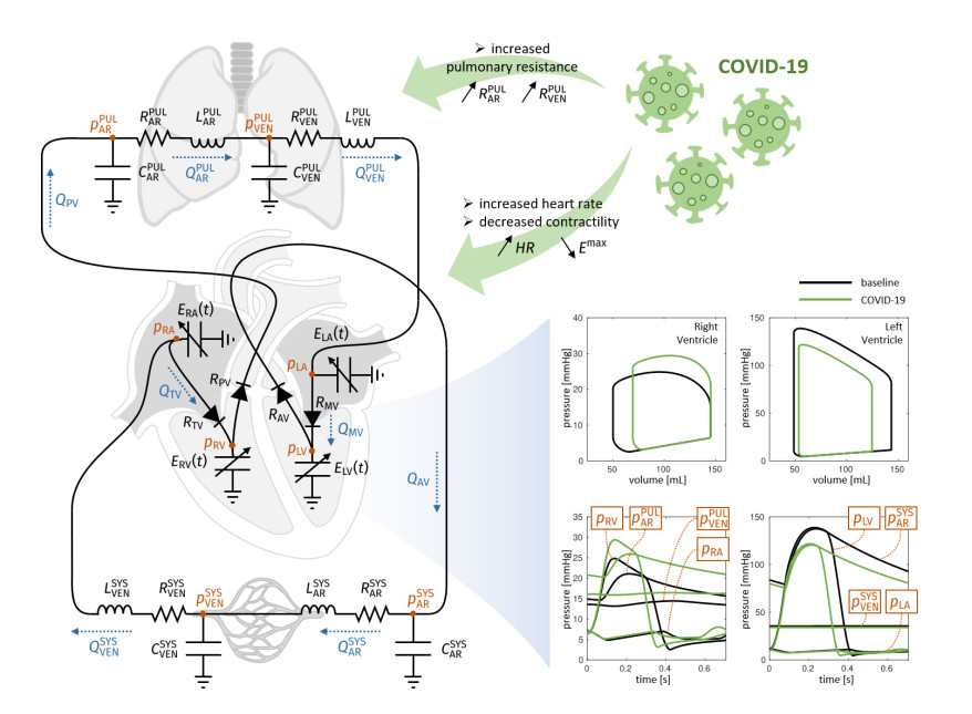
Emerging studies address how COVID-19 infection can impact the human cardiovascular system. This relates particularly to the development of myocardial injury, acute coronary syndrome, myocarditis, arrhythmia, and heart failure. Prospective treatment approach is advised for these patients. To study the interplay between local changes (reduced contractility), global variables (peripheral resistances, heart rate) and the cardiac function, we considered a lumped parameters computational model of the cardiovascular system and a three-dimensional multiphysics model of cardiac electromechanics. Our mathematical model allows to simulate the systemic and pulmonary circulations, the four cardiac valves and the four heart chambers, through equations describing the underlying physical processes. By the assessment of conventionally relevant parameters of cardiac function obtained through our numerical simulations, we propose a computational model to effectively reveal the interactions between the cardiac and pulmonary functions in virtual subjects with normal and impaired cardiac function at baseline affected by mild or severe COVID-19.
Citation: Luca Dedè, Francesco Regazzoni, Christian Vergara, Paolo Zunino, Marco Guglielmo, Roberto Scrofani, Laura Fusini, Chiara Cogliati, Gianluca Pontone, Alfio Quarteroni. Modeling the cardiac response to hemodynamic changes associated with COVID-19: a computational study[J]. Mathematical Biosciences and Engineering, 2021, 18(4): 3364-3383. doi: 10.3934/mbe.2021168
Emerging studies address how COVID-19 infection can impact the human cardiovascular system. This relates particularly to the development of myocardial injury, acute coronary syndrome, myocarditis, arrhythmia, and heart failure. Prospective treatment approach is advised for these patients. To study the interplay between local changes (reduced contractility), global variables (peripheral resistances, heart rate) and the cardiac function, we considered a lumped parameters computational model of the cardiovascular system and a three-dimensional multiphysics model of cardiac electromechanics. Our mathematical model allows to simulate the systemic and pulmonary circulations, the four cardiac valves and the four heart chambers, through equations describing the underlying physical processes. By the assessment of conventionally relevant parameters of cardiac function obtained through our numerical simulations, we propose a computational model to effectively reveal the interactions between the cardiac and pulmonary functions in virtual subjects with normal and impaired cardiac function at baseline affected by mild or severe COVID-19.

| [1] | M. Madjid, P. Safavi-Naeini, S. D. Solomon, O. Vardeny, Potential Effects of Coronaviruses on the Cardiovascular System—A Review, JAMA Cardiol., 5 (2020), 831-840. |
| [2] | T. Guo, Y. Fan, M. Chen, X. Wu, L. Zhang, T. He, et al., Cardiovascular Implications of Fatal Outcomesof Patients With Coronavirus Disease 2019 (COVID-19), JAMA Cardiol., 5 (2020), 811-818. |
| [3] | Q. Ruan, K. Yang, W. Wang, L. Jiang, J. Song, Clinical predictors of mortality due to COVID-19 based on an analysis of data of 150 patients from Wuhan, China, Intensive Care. Med., 46 (2020), 846-848. |
| [4] | F. Zhou, T. Yu, R. Du, G. Fan, Y. Liu, Z. Liu, et al., Clinical course and risk factors for mortality of adult inpatients with COVID-19 in Wuhan, China: a retrospective cohort study, Lancet, 395 (2020), 1054-1062. |
| [5] | A. Lala, K. W. Johnson, J. L. Januzzi, A. J. Russak, I. Paranjpe, F. Richter, et al., Prevalence and Impact of Myocardial Injury in Patients Hospitalized with COVID-19 Infection, JACC, 76 (2020), 533-546. |
| [6] | R. Kawakami, A. Sakamoto, K. Kawai, A. Gianatti, D. Pellegrini, A. Nasr, et al., Pathological evidence for SARS-CoV-2 as a cause of myocarditis: JACC review topic of the week, J. Am. Coll. Cardiol., 77 (2021), 314-325. |
| [7] | T. Mauri, E. Spinelli, E. Scotti, G. Colussi, M. C. Basile, S. Crotti, et al., Potential for Lung Recruitment and Ventilation-Perfusion Mismatch in Patients With Acute Respiratory Distress Syndrome From Coronavirus Disease 2019, Crit. Care Med., 48 (2020), 1129. |
| [8] | A. Quarteroni, L. Dede', A. Manzoni, C. Vergara, Mathematical Modelling of the Human Cardiovascular System - Data, Numerical Approximation, Clinical Applications, Cambridge University Press, (2019). |
| [9] | M. Olufsen, C. Peskin, W. Kim, E. Pedersen, A. Nadim, J. Larsen, Numerical simulation and experimental validation of blood flow in arteries with structured-tree outflow conditions, Ann. Biomed. Engrg., 28 (2000), 1281-1299. |
| [10] | A. Quarteroni, S. Ragni, A. Veneziani, Coupling between lumped and distributed models for blood flow problems, Comput. Vis. Sci., 4 (2001), 111-124, |
| [11] | L. G. Fernandes, P. R. Trenhago, R. A. Feijóo, P. J. Blanco, Integrated cardiorespiratory system model with short timescale control mechanisms, Int. J. Num. Meth. Biomed. Eng., (2020), e3332. |
| [12] | F. Regazzoni, M. Salvador, P. Africa, M. Fedele, L. Dede', A. Quarteroni, A cardiac electromechanics model coupled with a lumped parameters model for closed-loop blood circulation. Part I: model derivation, arXive, (2020), arXiv: 2011.15040. |
| [13] | F. Regazzoni, M. Salvador, P. Africa, M. Fedele, L. Dede', Quarteroni A, A cardiac electromechanics model coupled with a lumped parameters model for closed-loop blood circulation. Part II: numerical approximation, arXive, (2020), arXiv: 2011.15051. |
| [14] | A. Quarteroni, A. Veneziani, C. Vergara, Geometric multiscale modeling of the cardiovascular system, between theory and practice, Comput. Methods Appl. Mech. Eng., 302 (2016), 193-252. |
| [15] | A. Quarteroni, A. Manzoni, C. Vergara, The Cardiovascular System: Mathematical Modeling, Numerical Algorithms, Clinical Applications, Acta Numerica, 26 (2017), 365-590. |
| [16] | J. D. Bayer, R. C. Blake, G. Plank, N. Trayanova, A novel rule-based algorithm for assigning myocardial fiber orientation to computational heart models, Ann. Biomed. Eng., 40 (2012), 2243-2254. |
| [17] | K. H. Ten Tusscher, A. V. Panfilov, Alternans and spiral breakup in a human ventricular tissue model, Amer. J. Physiol.-Heart Circ. Physiol., 291 (2006), H1088-H1100. |
| [18] | P. C. Franzone, L. F. Pavarino, S. Scacchi, Mathematical Cardiac Electrophysiology, Vol. 13, Springer, 2014. |
| [19] | F. Regazzoni, L. Dedè, A. Quarteroni, Biophysically detailed mathematical models of multiscale cardiac active mechanics, PLoS Comput. Biol., 16 (2020), e1008294. |
| [20] | T. P. Usyk, I. J. LeGrice, A. D. McCulloch, Computational model of three-dimensional cardiac electromechanics, Comput. Vis. Sci., 4 (2002), 249-257. |
| [21] | A. Quarteroni, A. Valli, Numerical Approximation of Partial Differential Equations, Vol. 23, Springer Science & Business Media, 2008. |
| [22] | T. Y. Xiong, S. Redwood, B. Prendergast, M. Chen, Coronaviruses and the cardiovascular system: acute and long‐term implications, Eur. Heart J., 41 (2020), 1798-1800. |
| [23] | P. Qian-Yi, W. Xiao-Ting, Z. Li-Na, Chinese Critical Care Ultrasound Study Group (CCUSG). Using echocardiography to guide the treatment of novel coronavirus pneumonia, Crit. Care, 24 (2020), 143. |
| [24] | M. Hirschvogel, M. Bassilious, L. Jagschies, S. M. Wildhirt, M. W. Gee, A monolithic 3D-0D coupled closed-loop model of the heart and the vascular system: Experiment-based parameter estimation for patient-specific cardiac mechanics, Int. J. Num. Meth. Biomed. Eng., 33 (2017), e2842. |
| [25] | K. R. Walley, C. J. Becker, R. A. Hogan, K. Teplinsky, L. D. Wood, Progressive hypoxemia limits left ventricular oxygen consumption and contractility, Circ. Res., 63 (1998), 849-859. |
| [26] | J. Boehme, N. Le Moan, R. J. Kameny, A. Loucks, M. J. Johengen, A. L. Lesneski, et al., Preservation of myocardial contractility during acute hypoxia with OMX-CV, a novel oxygen delivery biotherapeutic, PLoS Biol., 16 (2018), e2005924. |
| [27] | R. M. Lang, L. P. Badano, V. Mor-Avi, J. Afilalo, A. Armstrong, L. Ernande, et al., Recommendations for Cardiac Chamber Quantification by Echocardiography in Adults: An Update from the American Society of Echocardiography and the European Association of Cardiovascular Imaging, Eur. Heart J. Cardiovasc. Imaging, 17 (2016), 412. |
| [28] | A. M. Maceira, S. K. Prasad, M. Khan, D. J. Pennell, Reference right ventricular systolic and diastolic function normalized to age, gender and body surface area from steady-state free precession cardiovascular magnetic resonance, Eur. Heart J., 27 (2006), 2879-2888. |
| [29] | A. Maceira, Normalized Left Ventricular Systolic and Diastolic Function by Steady State Free Precession Cardiovascular Magnetic Resonance, J. Cardiovasc. Magn. Reson., 8 (2006), 417-426. |
| [30] | P. A. Cain, R. Ahl, E. Hedstrom, M. Ugander, A. Allansdotter-Johnsson, P. Friberg, et al., Age and gender specific normal values of left ventricular mass, volume and function for gradient echo magnetic resonance imaging: a cross sectional study, BMC Med. Imaging, 9 (2009). |
| [31] | Y. Li, H. Li, S. Zhu, Y. Xie, B. Wang, L. He, et al., Prognostic Value of Right Ventricular Longitudinal Strain in Patients with COVID-19, Cardiovasc. Imaging, 13 (2020), 2287-2299. |
| [32] | S. Ghio, M. Guazzi, A. B. Scardovi, C. Klersy, F. Clemenza, E. Carluccio, et al., Different correlates but similar prognostic implications for right ventricular dysfunction in heart failure patients with reduced or preserved ejection fraction, Eur. J. Heart Fail., 19 (2017), 873-879. |
| [33] | E. Carluccio, P. Biagioli, G. Alunni, A. Murrone, C. Zuchi, S. Coiro, et al., Prognostic Value of Right Ventricular Dysfunction in Heart Failure With Reduced Ejection Fraction - Superiority of Longitudinal Strain Over Tricuspid Annular Plane Systolic Excursion, Circ. Cardiovasc. Imaging; 11 (2018), e006894. |
| [34] | H. A. Kontos, H. P. Mauck JR, D. W. Richardson, J. L. Patterson JR, Mechanism of circulatory responses to systemic hypoxia in the anesthetized dog, Am. J. Physiol-Legacy Content, 209 (1965), 397-403. |
| [35] | Zygote Solid 3D heart Generation II Development Report, Technical Report.2014. Available from: https://www.zygote.com/. |
| [36] | S. Heinke, C. Pereira, S. Leonhardt, M. Walter, Modeling a healthy and a person with heart failure conditions using the object-oriented modeling environment Dymola, Med. Biol. Eng. Comput., 53 (2015), 1049-1068. |
| [37] | T. Heldt, E. B. Shim, R. D. Kamm, R. G. Mark, Computational modeling of cardiovascular response to orthostatic stress, J. Appl. Physiol., 92 (2002), 1239-1254. |
| [38] | A. Albanese, L. Cheng, M. Ursino, N. W. Chbat, An integrated mathematical model of the human cardiopulmonary system: model development, Am. J. Physiol. Heart Circ. Physiol., 310 (2016), H899-H921. |
| [39] | C. Ngo, S. Dahlmanns, T. Vollmer, B. Misgeld, S. Leonhardt, An object-oriented computational model to study cardiopulmonary hemodynamic interactions in humans, Comput. Methods Programs Biomed., 159 (2018), 167-183. |
| [40] | K. Hemalatha, M. Manivannan, A study of Cardiopulmonary interaction haemodynamics with detailed lumped parameter model, Int. J. Biomed. Eng. Technol., 6 (2011), 251-271 |
| [41] | M. Busana, M. Schiavone, A. Lanfranchi, G. B. Forleo, E. Ceriani, C. B. Cogliati, et al., Non-invasive hemodynamic profile of early COVID‐19 infection, Physiol. Rep., 8 (2020), e14628. |
| [42] | S. Di Gregorio, M. Fedele, G. Pontone, A. F. Corno, P. Zunino, C. Vergara, et al., A multiscale computational model of myocardial perfusion in the human heart, J. Comput. Phys., 424 (2021), 109836. |
Figures(5) / Tables(4)

Luca Dedè, Francesco Regazzoni, Christian Vergara, Paolo Zunino, Marco Guglielmo, Roberto Scrofani, Laura Fusini, Chiara Cogliati, Gianluca Pontone, Alfio Quarteroni. Modeling the cardiac response to hemodynamic changes associated with COVID-19: a computational study[J]. Mathematical Biosciences and Engineering, 2021, 18(4): 3364-3383. doi: 10.3934/mbe.2021168


 DownLoad: