Stability and Hopf bifurcations in a competitive tumour-immune system with intrinsic recruitment delay and chemotherapy

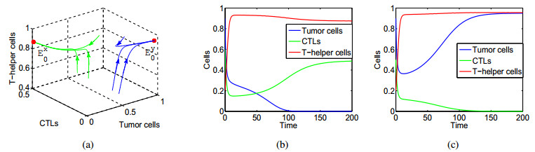
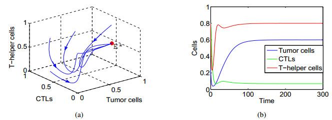
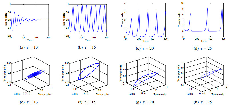
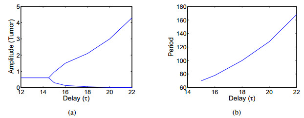
1.   Introduction

Cancer or malignant tumor results from uncontrolled growth of normal cells ^[1]. According to the report of World Health Organization, there are about 14.1 million new cancer cases and 8.2 million deaths in the world and it is expected that annual cancer cases will rise from 14 million in 2012 up to 22 million in the following two decades ^[2].

The immune system can monitor and protect the host from tumor evasion. However, the mechanisms of tumor evasion and immune response are still not completely understood. One of the adaptive immune responses is cell-mediated immunity(CMI). Cell-mediated immunity involves the production of cytotoxic T-lymphocytes (CTLs) and release of various cytokines in response to an antigen mediated by T-lymphocytes. CTLs are able to recognize and destroy tumor cells. The immune system can be classified into two subclasses, namely, the hunting cells (cytotoxic T lymphocytes) and the resting cells (T Helper cells). Most CTLs require cytokines from helper (resting) T-cells in order to be activated efficiently ^[3,4].

Different mathematical models have been constructed to understand the complex interaction between tumor and anti-tumor elements ^{[5,6,7,8,9,10,11]}. Kuznetsov et al. ^[12] proposed a classical tumor-immune model to explain the phenomena of "sneaking through" of the tumor and formation of a tumor "dormant state". Letellier et al. ^[13] found there exist chaotic attractor in a simple model of three competing cell populations (host, immune and tumour cells). Assia and Wang ^[14] investigated the effects of stochastic noises on tumors dynamics under treatment.

In ^[3], Sarkar et al. classified the immune system into two subclasses and proposed the following system

Here $M$, $N$ and $Z$ represent the densities of tumor cells, hunting predator cells (cytotoxic T-lymphocytes) and resting predator cells (T-Helper cells), respectively; $q$ is the conversion of normal cells to malignant ones (fixed input), $r_{1}$ is the growth rate of tumor cells, $k_{1}$ and $k_{2}$ are the maximum capacity of tumor cells and resting cells, respectively; $\alpha$ is the predation/destruction rate of tumor cells by the hunting cells, $\beta$ is the conversion rate of resting cells to hunting cells, $d$ is the natural death rate of hunting cells. The authors obtained some thresholds to control the malignant tumor growth.

In order to prolong the survival of patients it is essential to initiate a specific treatment regimen such as surgery, radiotherapy and chemotherapy ^{[15,16,17,18,19,20]}. Among various treatment methods, chemotherapy is very important and widely used in practice. However chemotherapy also has some side effects and it may kill the normal cells and immune cells ^[21,22]. Some mathematical models have been proposed to evaluate the effects of chemotherapy on tumor-immune dynamical behavior ^[23,24]. We also refer to ^[25] and the references therein for related works.

To derive more realistic models, recent papers ^{[26,27,28,29,30,31,32,33]} focus on delayed-induced oscillations in tumor-immune system dynamics to explain the short-term oscillations as well as long-term tumour relapse during the progress of the disease. Particularly, following ^[3], Subhas et al. ^[4] proposed the following tumor-immune competitive system with time delay

They neglect the fixed input term $q$ of tumor in original Eq (1.1) by assuming that the tumour cells are not benign but malignant. Another modification to original Eq (1.1) is that a discrete time delay is added to prescribe the convention time from resting predator cells to hunting predator cells. It is found in Eq (1.2) that the introduction of time delay can lead to appearance of periodic solution. Some other tumor immune models with time delay were investigated in ^[34,35].

Considering the necessary times for molecule production and proliferation, the authors of ^{[36,37,38,39]} introduced the intrinsic recruitment delay of tumor. In fact, as a type of special population, the growth of tumor also need supply of nutrition and food and thus there exist intrinsic recruitment delay. In this paper, based on the models of Sarkar et al. ^[3], when considering the intrinsic recruitment delay and the effects of chemotherapy, we propose a new deterministic model describing tumor-immune responses as

Here $c_{1}$ reflects the chemotherapy effect on the depletion rate of tumour cells, $c_{2}$ and $c_{3}$ represent the side effect of chemotherapy on the hunting predator cells and resting predator cells, respectively. The term $r_{1}M(1-\frac{M(t-\tau)}{k_{1}})$ describes the intrinsic recruitment of tumor and the positive time delay constant $\tau$ describes the necessary times for molecule production, proliferation, etc. We also modify the Eq (1.1) by adding the term $-\alpha_{2}MN$ in the second equation, which represents the loss of hunting predator cells due to competition and destructive influence of tumour cells and is an important characteristic of cancer^[12].

In order to simplify the analysis, we non-dimensionalize the Eq (1.3) by using the following re-scaling

After dropping the over bar notation for notational clarity, we obtain the following renormalization model

The rest of this paper is organized as follows. In Section 2, we obtain the non-negativity and boundeness of solutions of Eq (1.4). In Section 3, we study the existence and stability of possible steady states of the model. In Section 4, we study the changes in the stability of positive equilibrium though the Hopf bifurcation analysis. The direction and stability of the bifurcated periodic solution is also obtained. In Section 5, we carry out some numerical simulations and provide some biological interpretations. Conclusions and discussions are then presented in Section 6.

2.   Non-negativity and boundeness

In this section, we discuss the non-negativity and boundedness of the solutions of Eq (1.4). For $\tau > 0$, let $\mathcal{C} = \mathcal{C}([-\tau, 0], \mathbb{R}^{3}_{+})$ denote the Banach space of continuous function mapping the interval $[-\tau, 0]$ into $\mathbb{R}^{3}_{+}$ with the topology of uniform convergence. The initial conditions are given by

with $\phi_{i}(\xi)\geq 0$, $\xi\in[-\tau, 0]$ and $\phi_{i}(0) > 0 \; (i = 1, 2, 3)$.

Theorem 2.1. The solutions of Eq (1.4) satisfying the initial conditions Eq (2.1) are non-negative and ultimately bounded.

Proof. We first define the right-hand side function of Eq (1.4) as

where $K(t) = (K_{1}(t), K_{2}(t), K_{3}(t))^{T}$ and $K_{1}(t) = x$, $K_{2}(t) = y$, $K_{3}(t) = z.$ It is obvious that the function $G(t, K(t))$ is locally Lipschitz and by the standard theory of functional differential equation, we know that there exists a unique solution for a given initial conditions. To prove the non-negativity of solutions of Eq (1.4), we first prove the non-negativity over the time interval $[0, \tau]$. Considering the right-hand side functions of Eq (1.4) over the time interval $[0, \tau]$, we have

It follows that the solutions of Eq (1.4) remain nonnegative in $[0, \tau]$. Similarly, we can repeat the process over $[\tau, 2\tau]$ and so on by using the method of steps, it can be proved that for any finite interval $[0, t]$, the solutions of Eq (1.4) remains non-negative.

Now we consider the boundeness of the solutions. It follows from the non-negativity of the solutions and the first equation of Eq (1.4) that

Note that the solution is bounded for delay-logistic equation (refer to ^[41]). We know from Eq (2.2) and the comparison principle that $x(t)$ is ultimately bounded for any nonnegative initial conditions. Define a new variable $U(t) = y(t)+\dfrac{\rho}{\gamma}z(t)$, and let $d = \min\{k+m_{2}, m_{3}\}$. By the non-negativity of the solutions of Eq (1.4), we have

Taking $Q = \frac{\rho \mu_{2}}{4 \gamma}$, we know from Eq (2.3) and comparison principle that $\limsup\limits_{t\rightarrow\infty}U(t)\leq\dfrac{Q}{d}$. So the solutions of Eq (1.4) are ultimately bounded.

3.   Existence and stability of equilibria

In this section, we investigate the existence and stability of equilibria for Eq (1.4) as delay is absent, that is

Clearly, some of equilibria of Eq (3.1) can be obtained easily as follows:

● There always exists extinction equilibrium $E_{0}^{xyz}(0, 0, 0)$.

● If $m_{1} < \mu_{1}$, the Eq (3.1) exists immunity-free equilibrium $E_{0}^{yz}(\frac{\mu_{1}-m_{1}}{\mu_{1}}, 0, 0)$.

● If $m_{3} < \mu_{2}$, the Eq (3.1) exists axial equilibrium $E_{0}^{xy}(0, 0, \frac{\mu_{2}-m_{3}}{\mu_{2}})$.

● If $m_{1} > \mu_{1}$ and $m_{3} < \mu_{2}$, the Eq (3.1) exists equilibrium $E_{0}^{y}(\frac{\mu_{1}-m_{1}}{\mu_{1}}, 0, \frac{\mu_{2}-m_{3}}{\mu_{2}})$.

● If $\mu_{2}m_{2}+\rho m_{3} < \mu_{2}(\rho-k)$, the Eq (3.1) exists tumor-free equilibrium $E_{0}^{x}(0, y_{1}, z_{1})$, where

For the existence of coexistence equilibrium, we have the following theorem.

Theorem 3.1. If Eqs (3.6) and (3.7) hold, the Eq (3.1) exists a unique coexistence equilibrium $E^{*}(x^{*}, y^{*}, z^{*})$.

Proof. The coexistence equilibrium $E^{*}(x^{*}, y^{*}, z^{*})$ of Eq (3.1) satisfies the following equations:

From the first equation of (3.2), we have

Substituting Eq (3.3) into the third equation of (3.2) comes to

Substituting Eqs (3.3) and (3.4) into the second equation of (3.2) yields

It is easy to see from Eqs (3.3) and (3.4) that $y^{*} > 0, z^{*} > 0$ if and only if

which indicates that

It follows from Eq (3.5) that $x^{*} > 0$ if and only if

To study the stability of the equilibria above when $\tau = 0$, we evaluate the Jacobian matrix of Equation (3.1) to get

Theorem 3.2. If $m_{1} > \mu_{1}$ and $m_{3} > \mu_{2}$, then $E_{0}^{xyz}(0, 0, 0)$ is globally asymptotically stable.

Proof. It follows from Eq (3.8) that the characteristic equation of (3.1) at extinction equilibrium $E_{0}^{xyz}(0, 0, 0)$ is

It is easy to see that the eigenvalues are

So if $m_{1} > \mu_{1}$, and $m_{3} > \mu_{2}$, equilibrium $E_{0}^{xyz}(0, 0, 0)$ is locally asymptotically stable.

Now we prove the global stability of $E_{0}^{xyz}(0, 0, 0)$. Note that $m_{1} > \mu_{1}$ and $m_{3} > \mu_{2}$. It follows that $\frac{dx}{dt} < 0, \ \frac{dz}{dt} < 0,$ which implies that

Then from Eq (3.9) and the second equation of (3.1) we have

It follows from Eqs (3.9) and (3.10) that $E_{0}^{xyz}(0, 0, 0)$ is globally attractive. The proof is completed.

Theorem 3.3. Assume that $m_{1} < \mu_{1}$. If $m_{3} > \mu_{2}$, then $E_{0}^{yz}(\frac{\mu_{1}-m_{1}}{\mu_{1}}, 0, 0)$ is globally asymptotically stable.

Proof. It follows from Eq (3.8) that the characteristic equation of (3.1) at $E_{0}^{yz}(\frac{\mu_{1}-m_{1}}{\mu_{1}}, 0, 0)$ is

Clearly the eigenvalues

So if $\mu_{2} < m_{3}$, we have $\lambda_{3} = \mu_{2}-m_{3} < 0$. We know that $E_{0}^{yz}(\frac{\mu_{1}-m_{1}}{\mu_{1}}, 0, 0)$ is locally asymptotically stable.

Now we prove the global stability of $E_{0}^{yz}(\frac{\mu_{1}-m_{1}}{\mu_{1}}, 0, 0)$. It follows from $m_{3} > \mu_{2}$ that $\frac{dz}{dt} < 0$, which implies that

Then from Eq (3.11) and the second equation of (3.1), we have $\frac{dz}{dt} < 0$ for large $t$, which indicates that

There exists $T_{1}(\epsilon) > 0$ such that $0\leq y(t)\leq \epsilon$ as $t > T_{1}(\epsilon)$. Then from the first equation of (3.1), we have

It follow from Eq (3.13), comparison principle and the arbitrariness of $\epsilon$ that

We know from Eqs (3.11), (3.12) and (3.14) that $E_{0}^{yz}(\frac{\mu_{1}-m_{1}}{\mu_{1}}, 0, 0)$ is globally attractive. The proof is completed.

Theorem 3.4. Assume that $m_{3} < \mu_{2}$. If $m_{1} > \mu_{1}$ and $\mu_{2}m_{2}+\rho m_{3} > \mu_{2}(\rho-k)$, then $E_{0}^{xy}(0, 0, \frac{\mu_{2}-m_{3}}{\mu_{2}})$ is globally asymptotically stable.

Proof. It follows from Eq (3.8) that the characteristic equation of (3.1) at equilibrium $E_{0}^{xy}$ is

The eigenvalues are

So if $m_{1} > \mu_{1}$ and $\mu_{2}m_{2}+\rho m_{3} > \mu_{2}(\rho-k)$, $E_{0}^{xy}$ is locally asymptotically stable.

Now we prove the global stability of $E_{0}^{xy}(0, 0, \frac{\mu_{2}-m_{3}}{\mu_{2}})$. It follows from $m_{1} > \mu_{1}$ that $\frac{dx}{dt} < 0$, which implies that

From the third equation of (3.1) we have

which indicates that

Then from the second equation of (3.1) we have

for large $t$. Since $\mu_{2}m_{2}+\rho m_{3} > \mu_{2}(\rho-k)$, we have $\frac{dy}{dt} < 0$, which indicates that

There exists $T_{2}(\epsilon) > 0$ such that $0\leq y(t)\leq \epsilon$ as $t > T_{2}(\epsilon)$. It follows from the third equation of (3.1) that

which implies that

It follow from Eqs (3.16) and (3.18), the arbitrariness of $\epsilon$ that

Then from Eqs (3.15), (3.17) and (3.19), we know that $E_{0}^{xy}(0, 0, \frac{\mu_{2}-m_{3}}{\mu_{2}})$ is globally attractive. The proof is completed.

Theorem 3.5. Assume that $m_{1} < \mu_{1}$ and $m_{3} < \mu_{2}$. If $\mu_{2}m_{2}+\rho m_{3} > \mu_{2}(\rho-k)+\frac{\mu_{2}\alpha}{u_{1}}(m_{1}-\mu_{1})$, $E_{0}^{y}(\frac{\mu_{1}-m_{1}}{\mu_{1}}, 0, \frac{\mu_{2}-m_{3}}{\mu_{2}})$ is locally asymptotically stable.

Proof. It follow from Eq (3.8) that the characteristic equation of (3.1) at equilibrium $E_{0}^{y}$ is

where

Note that eigenvalues

since $m_{1} < \mu_{1}$ and $m_{3} < \mu_{2}$. Thus if eigenvalue $\lambda_{3} = \frac{A}{\mu_{1}\mu_{2}} < 0$, that is

the equilibrium $E_{0}^{y}$ is locally asymptotically stable.

Theorem 3.6. Assume that $\mu_{2}m_{2}+\rho m_{3} < \mu_{2}(\rho-k)$. If $\mu_{2}m_{2}+\rho m_{3} < \mu_{2}(\rho-k)+\rho\gamma(m_{1}-\mu_{1})$, then $E_{0}^{x}(0, y_{1}, z_{1})$ is locally asymptotically stable.

Proof. It follows from Eq (3.8) that the characteristic equation of (3.1) at tumor-free equilibrium $E_{0}^{x}(0, y_{1}, z_{1})$ is

One of the eigenvalues is

The other two eigenvalues $\lambda_{2}$ and $\lambda_{3}$ are determined by the following equation

Note that

Then the real parts of eigenvalues $\lambda_{2}$ and $\lambda_{3}$ are negative. So if $\lambda_{1} < 0$, that is

the tumor-free equilibrium $E_{0}^{x}(0, y_{1}, z_{1})$ is locally asymptotically stable.

Remark 3.7. It can be seen from Theorem 3.5 and Theorem 3.6 that there exist bistable phenomenon in the Eq (3.1). Both $E_{0}^{x}$ and $E_{0}^{y}$ are locally asymptotically stable if $m_{1} < \mu_{1}$, $m_{3} < \mu_{2}$ and

which indicates that if the tumor can be cleared or not depends on the initial densities of different types of cells.

Theorem 3.8. Assume that Eqs (3.6) and (3.7) hold. The coexistence equilibrium $E^{\ast}$ is locally asymptotically stable if and only if the following conditions hold:

Proof. It follows from Eq (3.8) that the characteristic equation of (3.1) at coexistence equilibrium $E^{\ast}$ is

where

Clearly $a_{1} > 0$. Then by Routh-Hurwitz Criterion, if $a_{3} > 0$ and $a_{1}a_{2}-a_{3} > 0$, that is the conditions $(H1)$ and $(H2)$ hold, $E^{\ast}$ is locally asymptotically stable.

Remark 3.9. It can be seen from Theorem 3.8 that if the destructive influence of tumor cells is small, that is $\alpha$ is small enough, the conditions $(H1)$ and $(H2)$ hold, and the coexistence equilibrium $E^{\ast}$ is locally asymptotically stable.

Theorem 3.10. If the coexistence equilibrium $E^{\ast}$ is asymptotically stable, all the other boundary equilibria are unstable.

Proof. If $E^{\ast}$ exist, we have $\mu_{1} > m_{1}$, $\mu_{2} > m_{3}$, which indicates that equilibria $E_{0}^{xyz}$, $E_{0}^{xy}$ and $E_{0}^{xy}$ can not be stable. It follows from Eq (3.6) that

which indicates that $E_{0}^{y}$ can not be stable. It follows from the stability of $E^{\ast}$ and Eq (3.7) that

which indicates that $E_{0}^{x}$ can not be stable.

Remark 3.11. It is believed that, although it is difficulty to complete the proof, the coexistence equilibrium $E^{\ast}$ is globally asymptotically stable when it is locally asymptotically stable. However, we can obtain the result about uniform persistence of Eq (3.1), which indicates that three types of cells can coexist.

Theorem 3.12. If the axial and planer singular points exist and

$(a)m_{1} < \mu_{1},$

$(b)m_{3} < \mu_{2}$,

$(c)\mu_{2}(\rho-k)+\rho\gamma(m_{1}-\mu_{1}) < \mu_{2}m_{2}+\rho m_{3} < \mu_{2}(\rho-k)+\frac{\mu_{2}\alpha}{\mu_{1}}(m_{1}-\mu_{1}),$

then the Eq (3.1) is uniformly persistent.

Proof. In order to prove the theorem we shall employ the method of average Lyapunov function ^[42]. Let us consider the following average Lyapunov function for the Eq (3.1)

where $\xi_{11}, \xi_{22}, \xi_{33}$ are all nonnegative constants to be chosen suitably in the subsequent steps. It can be noted that $\psi(x, y, z)$ is a positive continuous function defined in the positive quadrant $\bf{R}^{3}_{+}$. Taking the time derivative along the solution of Eq (3.1), we have

It is easy to show that the $\omega$-limit sets for Eq (3.1) on the boundary of the positive cone consists of fixed points. Thus to prove the uniform persistence of the Eq (3.1), it is sufficient to verify that $\Gamma(x, y, z)$ is positive for all singular points and the suitable choice of $\xi_{11}, \xi_{22}, \xi_{33} > 0$, that is, the following conditions must be satisfied:

and

Noting $\mu_{1}-m_{1} > 0$ and $\mu_{2}-m_{3} > 0$, we can take large $\xi_{11}$ and $\xi_{33}$ and small $\xi_{22}$ such that Eqs (3.20), (3.21) and (3.22) are satisfied. It follows that if

Equations (3.23) and (3.24) hold. The proof is completed.

Remark 3.13. It is found that if the effect of chemotherapy on depletion of tumor cells is strong enough ($m_{1} > \mu_{1}$), tumor cells would be cleared. While if the effect of chemotherapy is relatively weak ($m_{1} < \mu_{1}$), the dynamics of Eq (3.1) rely on the side effects of chemotherapy on the hunting predator cells $(m_{2})$ and resting predator cells $(m_{3})$, respectively. Then to control or clear the tumor, it is important to increase the effect of chemotherapy on tumor cells and let the side effect of chemotherapy on the predator cells be under a threshold.

4.   Hopf bifurcation

In this section, we take the discrete time delay $\tau$ as a bifurcation parameter and show that when $E^{\ast}$ loses its stability and a Hopf bifurcation occurs when the time delay passes through a critical value.

4.1.   Existence of Hopf bifurcation

In order to study the stability of the coexistence equilibrium $E^{\ast}$ of Eq (1.4), we first compute the Jacobian matrix as following

Then the characteristic equation at $E^{*}$ is

where

Putting $\lambda = i\omega$ into the characteristic Eq (4.1) and separating the real and imaginary parts, we have

and

Adding up the squares of the corresponding sides of Eqs (4.2) and (4.3) yields the following algebra equation with respect to $\omega$

where

Let $u = \omega^{2}$. Then Eq (4.4) becomes

If Eq (4.5) has a positive real root $u$, the characteristic Eq (4.1) has a purely imaginary root $i\omega = \sqrt{u}$; otherwise, Eq (4.1) has no purely imaginary root.

Note that

We have $p_{3} < 0$ if and only if (H1) is satisfied. We know that the stability of coexistence equilibrium $E^{*}$ as $\tau = 0$ implies that Eq (4.5) has at least one positive real root. If we further assume that $p_{2} < 0$, by Descartes sign rule, we know that Eq (4.5) has a unique positive real root $u_{0}$. In addition it can be shown that $Q'(u_{0}) > 0.$

Let $\omega_{0} = \sqrt{u_{0}}.$ It follows from Eqs (4.2) and (4.3) that

Then at increasing sequences of $\tau$ values,

Equation (4.1) has a pair of purely imaginary roots $\pm i\omega_{0}$.

Now, it remain to check the transversality condition required by the Hopf bifurcation theorem. Substituting $\lambda(\tau)$ into Eq (4.1) and differentiating the resulting equation in $\tau$, we obtain

Then we have

which indicates that

Since $Q'(u_{0}) > 0$, then for $j = 0, 1, 2, ...,$ we have

We know that at each $\tau_{j}$, $j = 0, 1, 2, \cdot\cdot\cdot,$ a pair of characteristic roots of Eq (4.1) cross the imaginary axis to the right. Then the transversality condition required by the Hopf bifurcation theorem is satisfied. We thus obtain the following result.

Theorem 4.1. Assume that the conditions in Theorem 3.8 hold.

(i) If $p_{2} > 0$, $E^{*}$ is locally asymptotically stable for $\tau\in[0, \tau_{0}]$ and unstable for $\tau > \tau_{0}$.

(ii) Equation (1.4) undergoes a Hopf bifurcation at $E^{*}$ when $\tau = \tau_{0}$. That is, Eq (1.4) has a branch of nonconstant periodic solutions bifurcating from $E^{*}$ near $\tau = \tau_{0}$.

4.2.   Direction and stability of the Hopf bifurcation

In the previous section, we studied the stability of the coexistence equilibrium $E^{*}$ of Eq (1.4) and the existence of Hopf bifurcations. We know Eq (1.4) has a branch of nonconstant periodic solutions bifurcating from $E^{*}$ near $\tau = \tau_{0}$. It is interesting to further determine the direction, stability of bifurcated periodic solutions.

Let $\mu = \tau-\tau_{0}$ and then $\mu = 0$ is the Hopf bifurcation value of Eq (1.4) at $E^{*}$. Introduce the change of variables

Let $\bar{x}_{i}(t) = x_{i}(\tau t)$ and drop the bars for simplicity of notation. Define operators $L(\mu):C\longrightarrow \mathbb{R}^{3}$ and $F(\mu, \phi):\mathbb{R}\times C\longrightarrow \mathbb{R}^{3}$ by

and

respectively, where $\phi(\theta) = (\phi_{1}(\theta), \phi_{2}(\theta), \phi_{3}(\theta))^{T}\in C$. Then Eq (1.4) may be transformed into a FDE in $C = C([-1, 0], \mathbb{R}^{3})$ as

where

By Riesz representation theorem, there exists bounded variation function $\eta(\theta, \mu):[-1, 0]\rightarrow \mathbb{ R}^{3}$ such that

where

and $\delta(\theta)$ is the Dirac delta function. For $\phi\in C([-1, 0], \mathbb{R}^{3})$, we define

and

Then Eq (4.7) is equivalent to the following operator equation

For $\varphi\in C([0, 1], (\mathbb{R}^{3})^{*})$, we define

For $\varphi\in C([0, 1], (\mathbb{R}^{3})^{*})$ and $\phi\in C([-1, 0], \mathbb{R}^{3})$, we define a bilinear form as

where $\eta(\theta) = \eta(\theta, 0)$. Then it is not difficult to show that $A^{\ast}(0)$ is the adjoint operator of $A(0)$. By the discussion at the beginning of this section, we know that $\pm i\omega_{0}\tau_{0}$ are eigenvalues of $A(0)$. Thus, they are also eigenvalues of $A^{*}(0)$.

Let $q(\theta) = (1, q_{2}, q_{3})^{\mathrm{T}}e^{i\omega_{0}\tau_{0}\theta}$ be the eigenvectors of matric $A$ corresponding to eigenvalue $i\omega_{0}\tau_{0}$. Then we have

It follows that

Let $q^{\ast}(s) = D(1, q^{\ast}_{2}, q^{\ast}_{3})^{\mathrm{T}}e^{i\omega_{0}\tau_{0}s}$ be the eigenvectors of matric $A^{\ast}$ corresponding to eigenvalue $-i\omega_{0}\tau_{0}$. Then we have

It follows that

Note that

Then we can choose

such that $< q^{\ast}(s), q(\theta) > = 1$.

Now following the standard notations and algorithms given in ^[44] and using a computation process similar to that of Wei and Ruan ^[43], we can obtain the following coefficients which will be used for determining the important qualities:

where $W_{11}^{(1)}(-1)$, $W_{20}^{(i)}(0)$ and $W_{11}^{(i)}(0)$ are given, respectively, by

and

Furthermore the constant vector $E_{20}$ satisfy the following equation

It follows that

The constant vector $E_{20}$ satisfy the following equation

It follows that

So far, we have calculated $g_{20}$, $g_{11}$, $g_{02}$, $g_{21}$ and then we can obtain

It is known that $\nu_{2}$ and $\beta_{2}$ will determine the direction and stability of the Hopf bifurcation, and $T_{2}$ determines the period of the bifurcated periodic solutions. In particular, if $\nu_{2} > 0(\nu_{2} < 0)$, the Hopf bifurcation is supercritical (subcritical) and the bifurcated periodic solutions exist for $\tau > \tau_{0}(\tau < \tau_{0})$. If $\beta_{2} < 0$($\beta_{2} > 0$), the bifurcated periodic solutions are stable(unstable). The period will become longer(shorter) if $T_{2} > 0$($T_{2} < 0$).

5.   Numerical simulations

In this section, we carry out some numerical simulations to display the qualitative behaviours of Eq (1.4) and confirm the theoretical results obtained in the above sections. We perform simulations by using MATLAB software with realistic parameter values given in Table 1.

According to the ranges of parameters in Table 1, we first take the following normalized parameter values

Then we obtain the boundary equilibria $E_{0}^{x} = (0, 0.49, 0.8750)$, $E_{0}^{y} = (0.95, 0, 0.9567)$. It is easy to check that the conditions in Theorems 3.5 and 3.6 are satisfied. Then both $E_{0}^{x}$ and $E_{0}^{y}$ are locally asymptotically stable and $E^{*}$ is unstable. Figure 1 presents a phase diagram and time series of the solutions of Eq (1.4). One can see that the trajectories converge to either $E_{0}^{x}$ or $E_{0}^{y}$ with different initial positions. Specially, when the initial density of hunting predator cells is small, the tumour cells tend to be persistent; when the initial density of hunting predator cells is relatively large, the tumour cells will be cleared.

To investigate the stability of coexistence equilibrium $E^{\ast}$, we choose a slightly different set of the normalized parameter values as following

The coexistence equilibrium is $E^{\ast} = (0.6, 0.07, 0.8)$. One can show that the conditions in Theorem 3.8 are satisfied and then $E^{\ast}$ is locally asymptotically stable when $\tau = 0$, which implies that all the boundary equilibria including $E_{0}^{x}$ and $E_{0}^{y}$ are unstable. One can see that the trajectories around $E^{*}$ converge to it (see Figure 2).

From Eq (4.6), we can obtain the Hopf bifurcation point $\tau_{0} = 14.5117$. By Eq (4.8), we obtain the Hopf bifurcation parameters $\nu_{2} = 40.3056$, $\beta_{2} = -0.3561$, $T_{2} = 5.8354$. Then we know that the Hopf bifurcation at $E^{\ast}$ is supercritical, the bifurcated periodic solutions is stable and the period will increase with the increase of time delay. Figure 3 gives the time series and phase diagrams of the solutions of Equation (1.4) with different time delays. One can see that when the time delay is under the threshold, that is $\tau = 14 < \tau_{0}$, $E^{*}$ is a stable focus(see Figure 3(a), (e)), which can explain the short-term oscillations in tumour sizes; when $\tau = 15, 20, 25 > \tau_{0}$, a branch of stable periodic solutions bifurcate from $E^{\ast}$ and the period become larger with the increase of $\tau$ (see Figure 3(b)–(d), 3(f)–(h)), which can explain the long-term tumour relapse.

Figure 4 presents the amplitude and period of the bifurcated periodic solutions of Eq (1.4) with respect to different time delay $\tau$. One can see that, larger intrinsic recruitment delay lead to larger amplitude and longer period of the bifurcated periodic solutions, which indicates that the period of tumor relapse become longer and then can provide us with a longer period to control or delete the tumor. Furthermore, with the increase of time delay, the minimum of the periodic tumor tends to zero, which indicates larger delay $\tau$ contributes to the control of tumor growth.

Figure 5 shows the sensitivity of state variable $x(t)$ (tumour cells) to the parameters $m_{1}$, $m_{2}$, $m_{3}$ and $\alpha$. The oscillation behaviour indicates that the tumour cells population is very sensitive in the early time intervals. Note that $\frac{\partial x}{\partial m_{1}} < 0$. We know that the increase of $m_{1}$ is beneficial to control and clear the tumor (see Figure 5(a)). On the other hand, the positivity of $\frac{\partial x}{\partial m_{i}}0$ ($i = 1, 2$) indicates that stronger side effect of chemotherapy on hunting predator cells and resting predator cells leads to increase of tumor cells (see Figure 5(b), (d)). The positivity of $\frac{\partial x}{\partial \alpha}$ implies that larger destructive influence of tumor cells is not conductive to the control of tumor. Here we have used the so called "direct approach" to find sensitivity functions of Eq (1.4) (refer to ^[40]).

6.   Conclusions and discussion

The long-term relapse phenomenon of tumor, that is the appearance of periodic solution in a system including tumor, is interesting for the control or deletion of tumor. In this paper, we construct a three-dimensional nonlinear delay differential system including Tumor cells, cytotoxic-T lymphocytes, T-helper cells with recruitment delay and chemotherapy to investigate long-term relapse phenomena of tumor.

We first show that the existence and stability of the equilibria are influenced by the effects of chemotherapy and destructive influence of tumor cells and the results are summarized in the following Table 2.

It is found that there exist bistable phenomenon in Eq (1.4). Both tumor-free equilibrium $E_{0}^{x}$ and $E_{0}^{y}$ are locally asymptotically stable at the same time, which indicates that if the tumour cells can be eradicated or not rely on the initial density of the hunting predator cells (see Figure 1). We point out that the bistable phenomenon appearing in this paper is a new dynamical behavior compared with the results in ^[27] and ^[28], which indicates that the introduction of chemotherapy and destructive influence of tumor cells can generate richer dynamics in tumor-immune system.

It is found that the coexistence equilibrium is locally asymptotically stable if the destructive influence of tumor cells is small enough (see Figure 2). We also show that the introduction of intrinsic recruitment delay of tumor can leads to the appearance of periodic solutions through Hopf bifurcation, which is a different factor that explain the long-term relapse phenomena of tumor compared with the factor in ^[27] and ^[28] (see Figure 3). We further investigate the direction and stability of bifurcated periodic solutions by applying normal form method and center manifold theory. Finally, by numerical simulations, it is shown that, with the increase of delay $\tau$, the amplitude and period of the bifurcated periodic solutions increase and the minimum of the periodic tumor cells tend to zero, which indicates that the increase of delay $\tau$ is beneficial to the control of the growth of tumor (see Figure 4). The sensitivity of tumour cells population to small perturbations in $m_{1}$, $m_{2}$, $m_{3}$ and $\alpha$ are also investigated. It follows that tumour cells is negatively proportion with increasing the parameter $m_{1}$ and is positively proportion with increasing the parameter $m_{2}$, $m_{3}$ and $\alpha$ and they are very sensitive in the early time intervals and the sensitivity decreases by time to be insensitive in the steady state (see Figure 5).

Some aspects of the problem remain to be examined and studied in the future. For instance, we plan to extend our analysis to global Hopf bifurcation analysis. Some other factors that influence the dynamics of tumor including the biological heterogeneity of tumor and the resistance to immunotherapy or chemotherapy may be investigated.

Acknowledgments

The authors thank the referees for their valuable comments and suggestions. This work is supported by the National Natural Science Foundation of P.R. China (11871403, 11701472), Fundamental Research Funds for the Central Universities (XDJK2020B050).

Conflict of interest

The authors declare no conflict of interest in this paper.