A novel semi-supervised multi-view clustering framework for screening Parkinson's disease

Xiaobo Zhang; Donghai Zhai; Yan Yang; Yiling Zhang; Chunlin Wang; Xiaobo Zhang; Donghai Zhai; Yan Yang; Yiling Zhang; Chunlin Wang

doi:10.3934/mbe.2020192

Mathematical Biosciences and Engineering

2020, Volume 17, Issue 4: 3395-3411. doi: 10.3934/mbe.2020192

Previous Article Next Article

Research article

A novel semi-supervised multi-view clustering framework for screening Parkinson's disease

1.
School of Information Science and Technology, Southwest Jiaotong University, Chengdu 611756, China
2.
National Engineering Laboratory of Integrated Transportation Big Data Application Technology, Southwest Jiaotong University, Chengdu 611756, China

Received: 20 January 2020 Accepted: 26 April 2020 Published: 30 April 2020

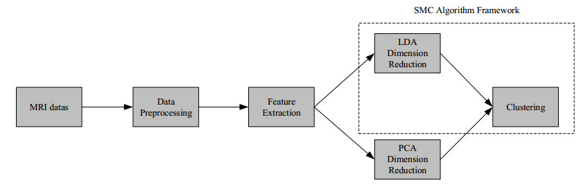
In recent years, there are many research cases for the diagnosis of Parkinson's disease (PD) with the brain magnetic resonance imaging (MRI) by utilizing the traditional unsupervised machine learning methods and the supervised deep learning models. However, unsupervised learning methods are not good at extracting accurate features among MRIs and it is difficult to collect enough data in the field of PD to satisfy the need of training deep learning models. Moreover, most of the existing studies are based on single-view MRI data, of which data characteristics are not sufficient enough. In this paper, therefore, in order to tackle the drawbacks mentioned above, we propose a novel semi-supervised learning framework called Semi-supervised Multi-view learning Clustering architecture technology (SMC). The model firstly introduces the sliding window method to grasp different features, and then uses the dimensionality reduction algorithms of Linear Discriminant Analysis (LDA) to process the data with different features. Finally, the traditional single-view clustering and multi-view clustering methods are employed on multiple feature views to obtain the results. Experiments show that our proposed method is superior to the state-of-art unsupervised learning models on the clustering effect. As a result, it may be noted that, our work could contribute to improving the effectiveness of identifying PD by previous labeled and subsequent unlabeled medical MRI data in the realistic medical environment.

Keywords:

Citation: Xiaobo Zhang, Donghai Zhai, Yan Yang, Yiling Zhang, Chunlin Wang. A novel semi-supervised multi-view clustering framework for screening Parkinson's disease[J]. Mathematical Biosciences and Engineering, 2020, 17(4): 3395-3411. doi: 10.3934/mbe.2020192

Related Papers:

[1]	Glenn Ledder . Incorporating mass vaccination into compartment models for infectious diseases. Mathematical Biosciences and Engineering, 2022, 19(9): 9457-9480. doi: 10.3934/mbe.2022440
[2]	Pannathon Kreabkhontho, Watchara Teparos, Thitiya Theparod . Potential for eliminating COVID-19 in Thailand through third-dose vaccination: A modeling approach. Mathematical Biosciences and Engineering, 2024, 21(8): 6807-6828. doi: 10.3934/mbe.2024298
[3]	Bruno Buonomo, Alberto d’Onofrio, Deborah Lacitignola . Rational exemption to vaccination for non-fatal SIS diseases: Globally stable and oscillatory endemicity. Mathematical Biosciences and Engineering, 2010, 7(3): 561-578. doi: 10.3934/mbe.2010.7.561
[4]	Beatriz Machado, Liliana Antunes, Constantino Caetano, João F. Pereira, Baltazar Nunes, Paula Patrício, M. Luísa Morgado . The impact of vaccination on the evolution of COVID-19 in Portugal. Mathematical Biosciences and Engineering, 2022, 19(1): 936-952. doi: 10.3934/mbe.2022043
[5]	Tetsuro Kobayashi, Hiroshi Nishiura . Prioritizing COVID-19 vaccination. Part 2: Real-time comparison between single-dose and double-dose in Japan. Mathematical Biosciences and Engineering, 2022, 19(7): 7410-7424. doi: 10.3934/mbe.2022350
[6]	Xiaojing Wang, Yu Liang, Jiahui Li, Maoxing Liu . Modeling COVID-19 transmission dynamics incorporating media coverage and vaccination. Mathematical Biosciences and Engineering, 2023, 20(6): 10392-10403. doi: 10.3934/mbe.2023456
[7]	Chuanqing Xu, Xiaotong Huang, Zonghao Zhang, Jing'an Cui . A kinetic model considering the decline of antibody level and simulation about vaccination effect of COVID-19. Mathematical Biosciences and Engineering, 2022, 19(12): 12558-12580. doi: 10.3934/mbe.2022586
[8]	ZongWang, Qimin Zhang, Xining Li . Markovian switching for near-optimal control of a stochastic SIV epidemic model. Mathematical Biosciences and Engineering, 2019, 16(3): 1348-1375. doi: 10.3934/mbe.2019066
[9]	Fang Wang, Lianying Cao, Xiaoji Song . Mathematical modeling of mutated COVID-19 transmission with quarantine, isolation and vaccination. Mathematical Biosciences and Engineering, 2022, 19(8): 8035-8056. doi: 10.3934/mbe.2022376
[10]	Yuto Omae, Yohei Kakimoto, Makoto Sasaki, Jun Toyotani, Kazuyuki Hara, Yasuhiro Gon, Hirotaka Takahashi . SIRVVD model-based verification of the effect of first and second doses of COVID-19/SARS-CoV-2 vaccination in Japan. Mathematical Biosciences and Engineering, 2022, 19(1): 1026-1040. doi: 10.3934/mbe.2022047

Abstract

1. Introduction

In the study of perturbations of the three degree of freedom Kepler Hamiltonian pulling back, the regularized Hamiltonian by the Kustaanheimo-Stiefel (KS) map, gives a perturbation of the four degree of freedom harmonic oscillator Hamiltonian, when restricted to the zero level set of the KS symmetry. We use the formulation of the KS transformation in ^[6] which allows us to reduce the KS symmetry using invariant theory for the first time. As an illustration, we apply this procedure to the regularized Stark Hamiltonian, which is normalized after applying the KS transformation. We do not expect this Hamiltonian to be completely integrable (see Lagrange ^[4] and also ^[5]). Our treatment follows that of ^[3] and gives the full details of obtaining the second order normal form ^[1]. We use the notation of ^[2] and note that our procedure of regularization, pull back by the KS map, normalization and reduction may be used to study three degree of freedom perturbed Keplerian systems.

2. The basic set up

On $T_0{\mathbb{R }}^3 = ({\mathbb{R }}^3\setminus \{ 0 \}) \times {\mathbb{R }}^3$ with coordinates $(x, y)$ and standard symplectic form ${\omega }_3 = \sum^3_{i = 1}\mathrm{d} x_i \wedge \mathrm{d} y_i$ consider the Stark Hamiltonian

$\begin{equation} K(x,y) = \tfrac{{ 1}}{{ 2}} \langle y, y \rangle -\frac{1}{|x|} + fx_3. \end{equation}$

(2.1)

Here, $\langle \, \, , \, \, \rangle$ is the Euclidean inner product on ${\mathbb{R} }^3$ with associated norm $|\, \, |$ . On the negative energy level $-\tfrac{ 1}{ 2} k^2$ with $k > 0$ rescaling time $\mathrm{d} t \mapsto \frac{|x|}{k}\mathrm{d} s$ , we obtain

$\begin{equation} 0 = \tfrac{1}{2k}\big( |x| \langle y,y \rangle +k^2|x|\big) -\frac{1}{k} + fx_3 \frac{|x|}{k}. \end{equation}$

(2.2)

In other words, $(x, y)$ lies in the $\tfrac{1}{k}$ level set of

$\begin{equation} \widehat{K}(x,y) = \tfrac{1}{2k}|x|\big( \langle y, y \rangle +k^2 |x| \big) + f x_3\frac{|x|}{k}. \end{equation}$

(2.3)

We assume that $f$ is small, namely, $f = \varepsilon \beta$ . After the symplectic coordinate change $(x, y) \mapsto (\frac{1}{k}x, ky)$ the Hamiltonian $\widehat{K}$ becomes the preregularized Hamiltonian

$\begin{equation} \mathcal{K}(x,y) = \tfrac{ 1}{ 2} |x|(\langle y, y \rangle +|x|) +\varepsilon \beta x_3|x| \end{equation}$

(2.4)

on the level set ${\mathcal{K}}^{-1}(1)$ .

Let $T_0{\mathbb{R} }^4 = ({\mathbb{R} }^4\setminus \{ 0 \}) \times {\mathbb{R} }^4$ have coordinates $(q, p)$ and a symplectic form ${\omega }_4 = \sum^4_{i = 1}\mathrm{d} q_i \wedge \mathrm{d} p_i$ . Pull back $\mathcal{K}$ by the Kustaanheimo-Stiefel mapping

$\mathcal{KS}: T_0{\mathbb{R} }^4 \rightarrow T_0{\mathbb{R} }^3: (q,p) \mapsto (x,y),$

where

$\begin{align*} x_1 & = 2(q_1q_3+q_2q_4) = U_2-K_1 \\ x_2 & = 2(q_1q_4-q_2q_3) = U_3 -K_2 \\ x_3 & = q^2_1+q^2_2-q^2_3-q^2_4 = U_4 - K_3 \\ y_1 & = (\langle q,q\rangle )^{-1}(q_1p_3+q_2p_4 +q_3p_1 +q_4p_2) = (H_2 + V_1)^{-1}V_2 \\ y_2 & = (\langle q,q\rangle )^{-1}(q_1p_4-q_2p_3 -q_3p_2 +q_4p_1) = (H_2 + V_1)^{-1}V_3 \\ y_3 & = (\langle q,q\rangle )^{-1}(q_1p_1+q_2p_2 -q_3p_3 -q_4p_4) = (H_2 + V_1)^{-1}V_4 \end{align*}$

and

$\begin{align*} H_2 & = \tfrac{ 1}{ 2} (p^2_1+p^2_2+p^2_3+p^2_4 +q^2_1+q^2_2 +q^2_3+q^2_4) \\ \Xi & = q_1p_2-q_2p_1 +q_3p_4 -q_4p_3, \end{align*}$

to get the regularized Stark Hamiltonian

$\begin{equation} \mathcal{H} = H_2 +\varepsilon \beta \big( U_4V_1+H_2U_4 -K_3V_1 -H_2K_3 \big) \end{equation}$

(2.5)

on ${\Xi}^{-1}(0)$ , since $|x| = \langle q, q \rangle = H_2+V_1$ . Here

$\begin{align} K_1 & = -(q_1q_3+q_2q_4+p_1p_3 +p_2p_4) \\ K_2 & = -(q_1q_4-q_2q_3+p_1p_4-p_2p_3) \\ K_3 & = \tfrac{ 1}{ 2} (q^2_3+q^2_4 +p^2_3+p^2_4 -q^2_1 -q^2_2 -p^2_1-p^2_2) \\ L_1 & = q_4p_1-q_3p_2+q_2p_3-q_1p_4 \\ L_2 & = q_1p_3+q_2p_4-q_3p_1-q_4p_2 \\ L_3 & = q_3p_4-q_4p_3+q_2p_1-q_1p_2 \\ U_1 & = -(q_1p_1+q_2p_2+ q_3p_3+ q_4p_4) \\ U_2 & = q_1q_3+q_2q_4-p_1p_3-p_2p_4 \\ U_3 & = q_1q_4 - q_2q_3 +p_2p_3 - p_1p_4 \\ U_4 & = \tfrac{ 1}{ 2} (q^2_1+q^2_2 -q^2_3 -q^2_4 +p^2_3 +p^2_4-p^2_1-p^2_2) \\ V_1 & = \tfrac{ 1}{ 2} (q^2_1+q^2_2 +q^2_3+q^2_4-p^2_1 -p^2_2-p^2_3-p^2_4) \\ V_2 & = q_1p_3 +q_2p_4 +q_3p_1 + q_4p_2 \\ V_3 & = q_1p_4 - q_2p_3 -q_3p_2 +q_4p_1 \\ V_4 & = q_1p_1 + q_2p_2 -q_3p_3 -q_4p_4. \end{align}$

generate the algebra of polynomials invariant under the $S^1$ action ${\varphi }^{\Xi}_s$ given by the flow of $X_{\Xi}$ on $(T{\mathbb{R} }^4 = {\mathbb{R} }^8, {\omega }_4)$ . The Hamiltonian $\mathcal{H}$ (2.5) is invariant under this $S^1$ action and thus is a smooth function on the orbit space ${\Xi}^{-1}(0)/S^1 \subseteq {\mathbb{R} }^{16}$ with coordinates $(K, L, H, {\Xi}; U, V)$ .

3. The first order normal form on ${\Xi}^{-1}(0)/S^1$

The harmonic oscillator vector field $X_{H_2}$ on $(T{\mathbb{R} }^4, {\omega }_4)$ induces the vector field $Y_{H_2} = \sum^4_{i = 1}\big(2V_i \frac{\partial }{\partial U_i} - 2U_i\frac{\partial }{\partial V_i }\big)$ on the orbit space ${\mathbb{R} }^8/S^1 \subseteq {\mathbb{R} }^{16}$ , which leaves ${\Xi}^{-1}(0)/S^1$ invariant.

We now compute the first order normal form of the Hamiltonian $\mathcal{H}$ (2.5) on the reduced space ${\Xi }^{-1}(0)/S^1 \subseteq {\mathbb{R} }^8/S^1$ .

The average of $H_2U_4-K_3V_1$ over the flow

${\varphi }^{Y_{H_2}}_t(K,L,H_2, \Xi ; U,V) = \big( K,L, H_2, \Xi ; U \cos 2t + V\sin 2t, -U\sin 2t + V \cos 2t \big)$

of $Y_{H_2}$ is

$\begin{align*} \overline{H_2U_4-K_3V_1} & = \tfrac{ 1}{ \pi} \int^{\pi }_0 ({\varphi }^{Y_{H_2}}_t)^{\ast }(H_2U_4 - K_3V_1 )\, \mathrm{d} t \\ & = \tfrac{ 1}{ \pi} \int^{\pi }_0 (U_4\cos 2t +V_4 \sin 2t) \mathrm{d} t \, H_2 - \tfrac{ 1}{ \pi} \int^{\pi }_0 (-U_1\sin 2t +V_1 \cos 2t) \mathrm{d} t \, K_3 = 0. \end{align*}$

The second equality above follows because $L_{X_{H_2}}K_3 = 0$ and the third because $\overline{\cos 2t} = \overline{\sin 2t } = 0$ . The average of $U_4V_1$ over the flow of $Y_{H_2}$ on ${\Xi }^{-1}(0)/S^1$ is

$\begin{align*} \overline{U_4V_1} & = \tfrac{ 1}{ \pi} \int^{\pi }_0 ({\varphi }^{Y_{H_2}}_t)^{\ast }(U_4V_1 )\, \mathrm{d} t \\ & = -\tfrac{ 1}{ 2} U_1U_4 \, \overline{\sin 4t} + U_4V_1\, \overline{{\cos }^2 \, 2t} - U_1V_4\, \overline{{\sin }^2 \, 2t} +\tfrac{ 1}{ 2} V_1V_4 \, \overline{\sin 4t} \\ & = \tfrac{ 1}{ 2} (U_4V_1 - U_1V_4) = -\tfrac{ 1}{ 2}H_2K_3, \end{align*}$

since $\overline{{\cos }^2 \, 2t} = \overline{{\sin }^2 \, 2t} = \tfrac{ 1}{ 2}$ and $\overline{\sin 4t} = 0$ . The last equality above follows from the explicit description of the orbit space ${\mathbb{R} }^8/S^1$ as the semialgebraic variety in ${\mathbb{R} }^{16}$ with coodinates $(K, L, U, V;H_2, \Xi)$ given by

$\begin{align} \langle U,U \rangle = U^2_1+U^2_2+U^2_3 +U^2_4 & = H^2_2 - {\Xi }^2 \ge 0 \, \, \, H_2 \ge 0 \\ \langle V,V \rangle = V^2_1+V^2_2+V^2_3 +V^2_4 & = H^2_2 - {\Xi }^2 \ge 0 \\ \langle U,V \rangle = U_1V_1 +U_2V_2+U_3V_3 + U_4V_4 & = 0 \\ U_2V_1-U_1V_2 & = L_1\Xi - K_1H_2 \\ U_3V_1-U_1V_3 & = L_2 \Xi - K_2H_2 \\ U_4V_1 - U_1V_4 & = L_3 \Xi -K_3H_2 \\ U_4V_3 -U_3V_4 & = K_1 \Xi -L_1H_2 \\ U_2V_4 -U_4V_2 & = K_2 \Xi -L_2H_2 \\ U_3V_2 -U_2V_3 & = K_3 \Xi -L_3H_2 . \end{align}$

(3.1)

So the average of $U_4V_1+ H_2U_4 - K_3V_1 - H_2K_3$ over the flow of $Y_{H_2}$ is $-\tfrac{ 3}{ 2}H_2K_3$ on ${\Xi }^{-1}(0)/S^1$ . Thus the first order normal form of the regularized Stark Hamiltonian $\mathcal{H}$ (2.5) on ${\Xi }^{-1}(0)/S^1$ is

$\begin{equation} {\mathcal{H}}^{(1)}_{\mathrm{nf}} = H_2 - \tfrac{ 3}{ 2} \beta \varepsilon H_2K_3. \end{equation}$

(3.2)

4. The second order normal form on ${\Xi }^{-1}(0)/S^1$

In order to compute the second order normal form of the Hamiltonian $\mathcal{H}$ on ${\Xi }^{-1}(0)/S^1$ , we need to find a function $F$ on ${\mathbb{R} }^{16}$ such that changing coordinates by the time $\varepsilon$ value of the flow of the Hamiltonian vector field $Y_F$ brings the regularized Hamiltonian $\mathcal{H}$ (2.5) into first order normal form. Choose $F$ so that

$\begin{equation} L_{Y_F}H_2 = \beta \big( -U_4V_1 - \tfrac{ 1}{ 2}H_2K_3 -H_2U_4 +K_3V_1 \big) . \end{equation}$

(4.1)

The following calculation shows that this choice does the job.

$\begin{align} ({\varphi }^{Y_F}_{\varepsilon })^{\ast }\mathcal{H} & = \mathcal{H} + \varepsilon L_{Y_F}\mathcal{H} + \tfrac{ 1}{ 2} {\varepsilon}^2 L^2_{Y_F}\mathcal{H} + \mathrm{O}({\varepsilon}^3) \\ & = H_2 +\varepsilon \beta \big( U_4V_1+H_2U_4-K_3V_1 -H_2K_3 \big) + \varepsilon L_{Y_F}H_2 \\ & +{\varepsilon }^2\beta L_{Y_F}\big( U_4V_1+ H_2U_4 -K_3V_1 -H_2K_3 \big) + \tfrac{ 1}{ 2} {\varepsilon }^2 L^2_{Y_F}H_2 + \mathrm{O}({\varepsilon }^3) \\ & = H_2 +\varepsilon \beta \big( U_4V_1+H_2U_4-K_3V_1 -H_2K_3 \big) \\ & + \varepsilon \beta \big( -U_4V_1 - \tfrac{ 1}{ 2}H_2K_3 -H_2U_4 + K_3V_1 \big) \\ & + {\varepsilon }^2 \big[ L_{Y_F}\big( -L_{Y_F}H_2 -\tfrac{ 3}{ 2}\beta H_2K_3 \big) +\tfrac{ 1}{ 2} L^2_{Y_F}H_2 \big] + \mathrm{O}({\varepsilon }^3) \\ & = H_2 -\tfrac{ 3}{ 2}\varepsilon \beta H_2K_3 -\tfrac{ 1}{ 2} {\varepsilon }^2\big( L^2_{Y_F}H_2 +3\beta L_{Y_F}(H_2K_3) \big) + \mathrm{O}({\varepsilon}^3). \end{align}$

(4.2)

To determine the function $F$ , we solve equation (4.1). Write $F = F_1+F_2$ , where $L_{Y_{H_2}}F_1 = \beta (U_4V_1+ \tfrac{ 1}{ 2} H_2K_3)$ and $L_{Y_{H_2}}F_2 = \beta (H_2U_4-K_3V_1)$ . Then

$\begin{align} L_{Y_F}H_2 & = -L_{Y_{H_2}}F = -L_{Y_{H_2}}F_1 - L_{Y_{H_2}}F_2 \\ & = -\beta (U_4V_1+ \tfrac{ 1}{ 2} H_2K_3) - \beta (H_2U_4-K_3V_1). \end{align}$

(4.3)

Since $L_{Y_{H_2}}V_4 = -2 U_4$ and $L_{Y_{H_2}}U_1 = 2V_1$ , it follows that

$\begin{equation} F_2 = - \tfrac{ \beta}{ 2}(H_2V_4 +K_3U_1). \end{equation}$

(4.4a)

Now

$\begin{align*} F_1 & = \tfrac{ \beta }{ \pi} \int^{\pi}_0 t({\varphi }^{Y_{H_2}}_t)^{\ast }\big( U_4V_1 + \tfrac{ 1}{ 2} H_2K_3 \big) \, \mathrm{d} t = \tfrac{ \beta}{ \pi} \int^{\pi}_0 t({\varphi }^{Y_{H_2}}_t)^{\ast }(U_4V_1) \mathrm{d} t + \tfrac{ \pi \beta }{ 4} H_2K_3, \end{align*}$

see ^[1], and

$\begin{align*} \tfrac{ \beta }{ \pi} \int^{\pi}_0 t({\varphi }^{Y_{H_2}}_t)^{\ast }(U_4V_1) \mathrm{d} t & = \\ & = -\tfrac{ \beta}{ 2}\ (U_1U_4) \, \tfrac{ 1}{ \pi} \int^{\pi }_0 t \, \sin 4t \mathrm{d} t + \beta (U_4V_1)\, \tfrac{ 1}{ \pi} \int^{\pi }_0 t \, {\cos }^2\, 2t \mathrm{d} t \\ &-\beta (U_1V_4)\, \tfrac{ 1}{ \pi} \int^{\pi }_0 t \, {\sin }^2\, 2t \mathrm{d} t + \tfrac{ \beta}{ 2} (V_1V_4)\, \tfrac{ 1}{ \pi} \int^{\pi }_0 t \, \sin 4t \mathrm{d} t \\ & = \tfrac{ \beta }{ 8} (U_1U_4 - V_1V_4) + \tfrac{ \pi \beta}{ 4}(U_4V_1 -U_1V_4) , \end{align*}$

since $\tfrac{1}{\pi } \int^{\pi}_0 t \, \sin 4t \mathrm{d} t = -\tfrac{1}{4}$ and $\tfrac{1}{\pi } \int^{\pi}_0 t \, {\sin }^2\, 2 t \mathrm{d} t = \tfrac{1}{\pi } \int^{\pi}_0 t \, {\cos }^2\, 2 t \mathrm{d} t = \tfrac{\pi }{4}$ . Thus

$\begin{equation} F_1 = \tfrac{ \beta}{ 8}(U_1U_4-V_1V_4) +\tfrac{ \pi \beta }{ 4} (U_4V_1 -U_1V_4 + H_2K_3) \notag \\ = \tfrac{ \beta }{ 8}(U_1U_4-V_1V_4) \label{eq-eightb} \end{equation}$

on ${\Xi}^{-1}(0)/S^1$ , see (3.1). Hence on ${\Xi}^{-1}(0)/S^1$

$\begin{equation} F = F_1+F_2 = \tfrac{ \beta }{ 8}(U_1U_4-V_1V_4) -\tfrac{ \beta}{ 2}(H_2V_4 + K_3U_1). \end{equation}$

(4.5)

We now calculate the average over the flow of $Y_{H_2}$ of

$\begin{equation} -\tfrac{ 3}{ 2}\beta L_{Y_F}(H_2K_3) -\tfrac{ 1}{ 2} L^2_{Y_F}H_2, \end{equation}$

(4.6)

which is the ${\varepsilon }^2$ term in the transformed Hamiltonian $({\varphi }^{Y_F}_{\varepsilon})^{\ast }\mathcal{H}$ , see (4.2). This determines the second order normal form of $\mathcal{H}$ on ${\Xi }^{-1}(0)/S^1$ . We begin with the term

$-\tfrac{ 3}{ 2} \beta L_{Y_F}(H_2K_3) = -\tfrac{ 3}{ 2}\beta [K_3(L_{Y_F}H_2) -H_2(L_{Y_{K_3}}F)] .$

The average of

$-\tfrac{ 3}{ 2} beta \, K_3(L_{Y_F}H_2) = \tfrac{ 3}{ 2}{\beta }^2\, K_3(U_4V_1 +\tfrac{ 1}{ 2} H_2K_3 + H_2U_4 -K_3V_1)$

vanishes on ${\Xi}^{-1}(0)/S^1$ . The term

$\begin{align*} \tfrac{ 3}{ 2}\beta H_2(L_{Y_{K_3}}F) & = \tfrac{ 3}{ 2}{\beta }^2H_2\, L_{Y_{K_3}}\big( \tfrac{ 1}{ 8}(U_1U_4-V_1V_4) -\tfrac{ 1}{ 2} (H_2V_4 +K_3U_1) \big) \\ & = \tfrac{ 3}{ 2}{\beta }^2 H_2 \big[ \big( -2L_2\frac{\partial }{\partial K_1} + 2L_1\frac{\partial }{\partial K_2} - 2K_2\frac{\partial }{\partial L_1} +2K_1\frac{\partial }{\partial L_2} \\ &-2U_4\frac{\partial }{\partial U_1} + 2U_1 \frac{\partial }{\partial U_4} -2V_4\frac{\partial }{\partial V_1} + 2V_1\frac{\partial }{\partial V_4 } \big) \big] \big( \tfrac{ 1}{ 8}(U_1U_4-V_1V_4) \\ &-\tfrac{ 1}{ 2} (H_2V_4 +K_3U_1) \big) , \, \, \mbox{see [2, table 1] } \\ & = \tfrac{ 3}{ 2} {\beta }^2H_2 \big[ \tfrac{ 1}{ 4} (-U^2_4+U^2_1+V^2_4-V^2_1) -H_2V_1 +K_3U_4 \big] . \end{align*}$

Next we calculate $\frac{ 3}{ 2}\beta \overline{H_2(L_{Y_{K_3}}F)}$ . Since $\overline{H_2V_1} = 0 = \overline{K_3U_4}$ we need only calculate the average of $U^2_1$ , $U^2_4$ , $V^2_1$ and $V^2_4$ . We get $\overline{U^2_1} = \tfrac{ 1}{ 2} (U^2_1+V^2_1) = \overline{V^2_1}$ and $\overline{U^2_4} = \tfrac{ 1}{ 2} (U^2_4+V^2_4) = \overline{V^2_4}$ . Thus $\tfrac{ 3}{ 2}\beta \overline{H_2(L_{Y_{K_3}}F)} = 0$ . So the average $-\tfrac{ 3}{ 2}\beta \overline{L_{Y_F}(H_2K_3)}$ of the first term in expression (4.6) vanishes on ${\Xi}^{-1}(0)/S^1$ .

Next we calculate the average of the term $L^2_{Y_F}H_2$ in expression (4.6) on ${\Xi }^{-1}(0)/S^1$ . We have

$\begin{align*} L^2_{Y_F}H_2 & = -L_{Y_F}(L_{Y_{H_2}}F) \\ & = -\beta L_{Y_F}\big( U_4V_1 + \tfrac{ 1}{ 2} H_2K_3 +H_2U_4 -K_3V_1) , \, \, \mbox{using (4.3)} \\ & = \beta \big[ \overbrace{(L_{Y_{U_4}}F)V_1}^{I} + \overbrace{U_4(L_{Y_{V_1}}F)}^{II} -\tfrac{ 1}{ 2} \overbrace{(L_{Y_F}H_2)K_3}^{III} + \tfrac{ 1}{ 2} \overbrace{H_2(L_{Y_{K_3}}F)}^{IV} \\ & -\overbrace{(L_{Y_F}H_2)U_4}^{V} + \overbrace{H_2(L_{Y_{U_4}}F)}^{VI} - \overbrace{(L_{Y_{K_3}}F)V_1}^{VII} -\overbrace{K_3(L_{Y_{V_1}}F)}^{VIII} \big] . \end{align*}$

We begin by finding

$\begin{align*} L_{Y_{H_2}}F & = \beta \big[ \big( 2V_1 \frac{\partial }{\partial U_1} + 2V_2 \frac{\partial }{\partial U_2} +2V_3 \frac{\partial }{\partial U_3} + 2V_4 \frac{\partial }{\partial U_4} -2U_1 \frac{\partial }{\partial V_1} - 2U_2 \frac{\partial }{\partial V_2} \\ & - 2U_3 \frac{\partial }{\partial V_3} -2U_4 \frac{\partial }{\partial V_4} \big) \big] \big( \tfrac{ 1}{ 8}(U_1U_4-V_1V_4) -\tfrac{ 1}{ 2} (H_2V_4 + K_3U_1) \big) \\ & = \beta \big[ \tfrac{ 1}{ 2}(V_1U_4+U_1V_4) +H_2U_4 - K_3V_1 \big] ; \\ L_{Y_{K_3}}F & = \beta \big( \big( -2L_2 \frac{\partial }{\partial K_1} + 2L_1 \frac{\partial }{\partial K_2} -2K_2 \frac{\partial }{\partial L_1} + 2K_1 \frac{\partial }{\partial L_2} -2U_4 \frac{\partial }{\partial U_1} + 2U_1 \frac{\partial }{\partial U_4} \\ & - 2V_4 \frac{\partial }{\partial V_1} +2V_1 \frac{\partial }{\partial V_4} \big) \big( \tfrac{ 1}{ 8}(U_1U_4-V_1V_4) -\tfrac{ 1}{ 2} (H_2V_4+K_3U_1) \big) \big) \\ & = \beta \big[ \tfrac{ 1}{ 4}(-U^2_4 +U^2_1 +V^2_4 - V^2_1) -H_2V_1 +K_3U_4 \big] ; \\ L_{Y_{U_4}}F & = \beta \big[ \big( -2U_1 \frac{\partial }{\partial K_3} - 2U_3 \frac{\partial }{\partial L_1} +2U_2 \frac{\partial }{\partial L_2} - 2V_4 \frac{\partial }{\partial H_2} -2K_3 \frac{\partial }{\partial U_1} + 2L_2 \frac{\partial }{\partial U_2} \\ & + 2V_3 \frac{\partial }{\partial U_3} - 2H_2 \frac{\partial }{\partial V_4} \big) \big( \tfrac{ 1}{ 8}(U_1U_4-V_1V_4) -\tfrac{ 1}{ 2} (H_2V_4+K_3U_1) \big) \big] \\ & = \beta \big[ V^2_4 +K^2_3 -\tfrac{ 1}{ 4}(K_3U_4 - H_2V_1) +H^2_2 + U^2_1\big] ; \\ L_{Y_{V_1}}F & = \beta \big[ \big( 2V_2 \frac{\partial }{\partial K_1} + 2V_3 \frac{\partial }{\partial K_2} +2V_4 \frac{\partial }{\partial K_3} + 2U_1 \frac{\partial }{\partial H_2} +2H_2 \frac{\partial }{\partial U_1} + 2K_1 \frac{\partial }{\partial V_2} \\ & + 2K_2 \frac{\partial }{\partial V_3} + 2K_3 \frac{\partial }{\partial V_4} \big) \big( \tfrac{ 1}{ 8}(U_1U_4-V_1V_4) -\tfrac{ 1}{ 2} (H_2V_4+K_3U_1) \big) \big] \\ & = \beta [-2(U_1V_4+H_2K_3) + \tfrac{ 1}{ 4}(H_2U_4-K_3V_1)] . \end{align*}$

So the average of term I on ${\Xi}^{-1}(0)/S^1$ is

$\begin{align} \beta \overline{(L_{Y_{U_4}}F)V_1} & = {\beta }^2(\overline{V_1V^2_4} + \overline{K^2_3V_1} -\tfrac{ 1}{ 4}\overline{K_3U_4V_1} + \tfrac{ 1}{ 4}\overline{H_2V^2_1} +\overline{H^2_2V_1} + \overline{U^2_1V_1}) \\ & = {\beta }^2 \big( \tfrac{ 1}{ 8}H_2K^2_3 + \tfrac{ 1}{ 8}H_2(U^2_1+V^2_1) \big) , \end{align}$

(4.7a)

since the average of $V_1V^2_4$ , $K^2_3V_1$ , $H^2_2V_1$ , and $U^2_1V_1$ are each $0$ , $\overline{U_4V_1} = -\tfrac{ 1}{ 2} H_2K_3$ and $\overline{V^2_1} = \tfrac{ 1}{ 2} (U^2_1+V^2_1)$ .

Term II is

$\beta U_4(L_{Y_{V_1}}F) = {\beta }^2 \big( - 2U_1U_4V_4 - 2H_2K_3U_4 + \tfrac{ 1}{ 4} H_2U^2_4 - \tfrac{ 1}{ 4}K_3U_4V_1 \big) .$

$\begin{align} \beta \overline{U_4(L_{Y_{V_1}}F)} & = \tfrac{ 1}{ 4} {\beta }^2 H_2 \overline{U^2_4} - \tfrac{ 1}{ 4} {\beta }^2 \, K_3 \overline{U_4V_1} \\ & = \tfrac{ 1}{ 8} {\beta }^2 H_2(U^2_4+V^2_4) + \tfrac{ 1}{ 8} {\beta }^2 H_2K^2_3. \end{align}$

(4.7b)

For term III, we have already shown that

$\begin{equation} -\tfrac{ \beta}{ 2}\overline{(L_{Y_F}H_2)K_3} = 0. \end{equation}$

(4.7c)

and for term IV we have already shown that

$\begin{equation} \tfrac{ \beta}{ 2}\overline{H_2(L_{Y_{K_3}}F)} = 0. \end{equation}$

(4.7d)

Term V is

$-{\beta }(L_{Y_F}H_2)U_4 = {\beta }^2 \big( \tfrac{ 1}{ 2} U^2_4V_1 + \tfrac{ 1}{ 2} U_1U_4V_1 + H_2U^2_4 - K_3U_4V_1 \big) .$

$\begin{align} -{\beta }\overline{(L_{Y_F}H_2)U_4} & = {\beta }^2 \big( \tfrac{ 1}{ 2} \overline{U^2_4V_1} + \tfrac{ 1}{ 2} \overline{U_1U_4V_1} + \overline{H_2U^2_4} - \overline{K_3U_4V_1} \big) \\ & = \tfrac{ {\beta }^2}{ 2} H_2 (U^2_4 + V^2_4) - \tfrac{ {\beta }^2}{ 2}K_3(U_4V_1 - U_1V_4), \end{align}$

(4.7e)

since the average of $U^2_4V_1$ and $U_1U_4V_1$ vanish; while $\overline{U^2_4} = \tfrac{ 1}{ 2} (U^2_4+V^2_4)$ and $\overline{U_4V_1} = \tfrac{ 1}{ 2} (U_4V_1 - U_1V_4)$ .

Term VI is

$\beta H_2(L_{Y_{U_4}}F) = {\beta }^2H_2\big( V^2_4 +K^2_3 - \tfrac{ 1}{ 4}K_3U_4 + \tfrac{ 1}{ 4} H_2V_1 +H^2_2 + U^2_1 \big) .$

$\begin{align} \beta \overline{H_2(L_{Y_{U_4}}F)} & = {\beta }^2 \, H_2\overline{V^2_4} +{\beta }^2\, H_2K^2_3 + {\beta }^2\, H^3_2 + {\beta }^2\, H_2 \overline{U^2_1} \\ & = \tfrac{ 1}{ 2} {\beta }^2\, H_2(U^2_4+V^2_4) + {\beta }^2H_2K^2_3 +{\beta }^2H^3_2 + \tfrac{ 1}{ 2} {\beta }^2\, H_2(U^2_1+V^2_1), \end{align}$

(4.7f)

since $\overline{K_2U_4} = 0 = \overline{H_2V_1}$ .

Term VII is

$-\beta (L_{Y_{K_3}}F)V_1 = {\beta }^2\big( \tfrac{ 1}{ 4}[U^2_4V_1-U^2_1V_1-V_1V^2_4 +V^3_1] +H_2V^2_1 - K_3U_4V_1 \big) .$

$\begin{align} -\beta \overline{(L_{Y_{K_3}}F)V_1} & = {\beta }^2 H_2\overline{V^2_1} - {\beta }^2K_3 \overline{U_4V_1} \\ & = \tfrac{ {\beta }^2}{ 2} H_2(U^2_1+V^2_1) - \tfrac{ {\beta }^2}{ 2} K_3(U_4V_1 - U_1V_4). \end{align}$

(4.7g)

Term VIII is

$-\beta K_3(L_{Y_{V_1}}F) = {\beta }^2\big( 2K_3 U_1V_4 + 2H_2K^2_3 - \tfrac{ 1}{ 4} H_2K_3 U_4 + \tfrac{ 1}{ 4} K^2_3V_1 \big) .$

$\begin{equation} -\beta \overline{K_3(L_{Y_{V_1}}F)} = 2{\beta }^2K_3\overline{U_1V_4} + 2{\beta }^2\, H_2K^2_3 = 3{\beta }^2\, H_2K^2_3, \end{equation}$

(4.7h)

since $\overline{U_1V_4} = \tfrac{ 1}{ 2} H_2K_3$ . Collecting together the results of all the above term calculations gives

$\begin{align*} \overline{L^2_{Y_F}H_2} & = \beta \overline{(L_{Y_{U_4}}F)V_1} + \beta \overline{U_4(L_{Y_{V_1}}F)} - \beta \overline{(L_{Y_F}H_2)U_4} +{\beta } \overline{H_2(L_{Y_{U_4}}F)} \\ & -{\beta }\overline{(L_{Y_{K_3}}F)V_1} - \beta \overline{K_3(L_{Y_{V_1}}F)} \\ & = {\beta }^2\big( [ \tfrac{ 1}{ 8}H_2K^2_3 + \tfrac{ 1}{ 8}H_2(U^2_1+V^2_1) ] + [\tfrac{ 1}{ 8} H_2(U^2_4+V^2_4) + \tfrac{ 1}{ 8} H_2K^2_3] \\ &+ [ \tfrac{ 1}{ 2} H_2(U^2_4+V^2_4) - \tfrac{ 1}{ 2} K_3(U_4V_1 -U_1V_4) ] + [ \tfrac{ 1}{ 2} H_2(U^2_4+V^2_4) + H_2K^2_3 + H^3_2 \\ & + \tfrac{ 1}{ 2} H_2(U^2_1+V^2_1)] + [ \tfrac{ 1}{ 2} H_2(U^2_1+V^2_1) - \tfrac{ 1}{ 2} K_3(U_4V_1-U_1V_4)] + 3 H_2 K^2_3 \big) \\ & = {\beta }^2 \big[ \tfrac{ 21}{ 4} H_2K^2_3 +H^3_2 + \tfrac{ 9}{ 8} H_2(U^2_1+V^2_1) + \tfrac{ 9}{ 8} H_2(U^2_4+V^2_4) \big] , \end{align*}$

using $U_4V_1-U_1V_4 = -K_3H_2$ . Thus the second order normal form of the regularized Stark Hamiltonian $\mathcal{H}$ on ${\Xi }^{-1}(0)/S^1$ is

$\begin{align} {\mathcal{H}}^{(2)}_{\mathrm{nf}} & = H_2 -\tfrac{ 3}{ 2} \varepsilon \beta H_2K_3 - \tfrac{ 1}{ 2} {\varepsilon }^2 \overline{L^2_{Y_F}H_2} = H_2 -\tfrac{ 3}{ 2}\varepsilon \beta H_2K_3 \\ & -\tfrac{ 1}{ 2} {\varepsilon }^2 {\beta }^2 H_2 \big[ \tfrac{ 21}{ 4} K^2_3 +H^2_2 + \tfrac{ 9}{ 8} (U^2_1+V^2_1) +\tfrac{ 9}{ 8} (U^2_4+V^2_4) \big] . \end{align}$

(4.8)

5. The first order normal form of ${\mathcal{H}}^{(2)}_{\mathrm{nf}}$ on $T_hS^3_1$

Since $L_{X_{H_2}}{\mathcal{H}}^{(2)}_{\mathrm{nf}} = 0$ by construction, the second order normal form ${\mathcal{H}}^{(2)}_{\mathrm{nf}}$ (4.8) is a smooth function on $(H^{-1}_2(h) \cap {\Xi}^{-1}(0))/S^1 = T_hS^3_1$ , the tangent $h$ -sphere bundle of the unit $3$ -sphere $S^3_1$ , given by

$\begin{align} \widetilde{\mathcal{H}} & = h - \tfrac{ 1}{ 2} {\varepsilon }^2{\beta }^2 h^3 - \tfrac{ 3}{ 2} \varepsilon \beta h K_3 \\ & - \tfrac{ 1}{ 2} {\varepsilon }^2{\beta }^2 h \big[ \tfrac{ 21}{ 4} K^2_3 + \tfrac{ 9}{ 8} (U^2_1+V^2_1) + \tfrac{ 9}{ 8} (U^2_4+V^2_4) \big] . \end{align}$

(5.1)

We now show that the Hamiltonian $\widetilde{\mathcal{H}}$ (5.1) on $T_hS^3_1$ can be normalized again. On $(T{\mathbb{R} }^4, {\omega }_4)$ the Hamiltonian

$K_3(q,p) = \tfrac{ 1}{ 2} (q^2_3+q^2_4+p^2_3+p^2_4-q^2_1-q^2_2-p^2_1-p^2_2)$

gives rise to the Hamiltonian vector field $X_{K_3}$ , whose flow ${\varphi }^{X_{K_3}}_t(q, p)$ is

$\begin{align*} &\big( q_1 \cos t -p_1\sin t, q_2\cos t -p_2 \sin t, q_3 \cos t + p_3 \sin t , q_4 \cos t +p_4 \sin t ,\\ &q_1 \sin t +p_1 \cos t, q_2 \sin t +p_2 \cos t, -q_3\sin t +p_3 \cos t, -q_4 \sin t + p_4\cos t \big) , \end{align*}$

which is periodic of period $2\pi$ .

The vector field $X_{K_3}$ on $T{\mathbb{R} }^4$ induces the vector field

$\begin{align*} Y_{K_3} & = -2L_2 \frac{\partial }{\partial K_1} +2L_1 \frac{\partial }{\partial K_2} -2K_2 \frac{\partial }{\partial L_1} +2K_1\frac{\partial }{\partial L_2 } \\ & - 2U_4\frac{\partial }{\partial U_1} + 2U_1 \frac{\partial }{\partial U_4} -2V_4\frac{\partial }{\partial V_1} + 2V_1 \frac{\partial }{\partial V_4} , \end{align*}$

on ${\Xi}^{-1}(0)/S^1 \subseteq {\mathbb{R} }^{16}$ with coordinates $(K, L, H_2, \Xi; U, V)$ , whose flow

$\begin{align*} {\varphi }^{Y_{K_3}}_s(K,L,H_2, \Xi ; U, V) & = \big( -L_2 \sin 2s + K_1 \cos 2s, L_1 \sin 2s +K_2 \cos 2s, K_3 \\ & -K_2\sin 2s +L_1\cos 2s , K_1 \sin 2s + L_2 \cos 2s, L_3, H_2, \Xi ; U_1 \cos 2s -U_4 \sin 2s, \\ &U_2, U_3, U_1 \sin 2s +U_4 \cos 2s, V_1 \cos 2s - V_4 \sin 2s, V_2, V_3, V_1\sin 2s + V_4 \cos 2s \big) \end{align*}$

is periodic of period $\pi$ . Since $L_{Y_{K_3}}$ maps the ideal of smooth functions which vanish identically on ${\Xi}^{-1}(0)/S^1$ into itself, $Y_{K_3}$ is a vector field on ${\Xi}^{-1}(0)/S^1$ . Since $L_{X_{K_3}}H_2 = 0$ , it follows that $Y_{K_3}$ induces a vector field on $T_hS^3_1$ with periodic flow. So we can normalize again.

To compute the normal form of the Hamiltonian $\widetilde{\mathcal{H}}$ (5.1) on $T_hS^3_1$ we need only calculate the average of the term

$T = \tfrac{ 21}{ 4} K^2_3 + \tfrac{ 9}{ 8} (U^2_1+V^2_1) +\tfrac{ 9}{ 8} (U^2_4+V^2_4)$

over the flow ${\varphi }^{Y_{K_3}}_s$ . Since $L_{Y_{K_3}}K_3 = 0$ , we need only calculate $\overline{U^2_1}$ , $\overline{U^2_4}$ , $\overline{V^2_1}$ , and $\overline{V^2_4}$ . Now

$\begin{align*} \overline{U^2_1} & = \tfrac{ 1}{ \pi} \int^{\pi }_0 (U_1 \cos 2s -U_4 \sin 2s)^2 \, \mathrm{d} s \\ & = \tfrac{ 1}{ \pi} \int^{\pi }_0 \big( U^2_1 {\cos }^2\, 2s - U_1U_4\sin 4s + U^2_4 {\sin }^2\, 2s \big) \mathrm{d} s = \tfrac{ 1}{ 2} (U^2_1+U^2_4). \end{align*}$

Similarly, $\overline{V^2_1} = \tfrac{ 1}{ 2} (V^2_1+V^2_4)$ , $\overline{U^2_4} = \tfrac{ 1}{ 2} (U^2_1+U^2_4)$ , and $\overline{V^2_4} = \tfrac{ 1}{ 2} (V^2_1+V^2_4)$ . Thus

$\begin{align} \overline{T} & = \tfrac{ 21}{ 4} K^2_3 + \tfrac{ 9}{ 8} h(U^2_1+V^2_1 +U^2_4+V^2_4) , \end{align}$

(5.2)

which is no surprise since $L_{Y_{K_3}}T = 0$ . So the first order normal form of $\widetilde{\mathcal{H}}$ (5.1) on $T_hS^3_1$ is

$\begin{align} {\widetilde{\mathcal{H}}}^{(1)}_{\mathrm{nf}} & = h - \tfrac{ 1}{ 2} {\varepsilon}^2 {\beta }^2h^3 - \tfrac{ 3}{ 2} \varepsilon \beta h K_3 \\ & - {\varepsilon }^2 {\beta }^2 h [ \tfrac{ 21}{ 8} K^2_3 + \tfrac{ 9}{ 16} (U^2_1+V^2_1+U^2_4+V^2_4)] . \end{align}$

(5.3)

6. The reduced Hamiltonian ${\widetilde{\mathcal{H}}}^{(1)}_{\mathrm{nf}}$ on $S^2_h\times S^2_h$

The polynomial $U^2_1+V^2_1 +U^2_4+V^2_4$ is invariant under the flows ${\varphi }^{X_{H_2}}_t$ , ${\varphi }^{X_{\Xi }}_u$ , and thus is a polynomial on the orbit space $T_hS^3_1/S^1 = S^2_h \times S^2_h$ , defined by

$\begin{align*} K^2_1+K^2_2+K^2_3 + L^2_1+L^2_2+L^2_3 & = h^2 \\ K_1L_1 +K_2L_2 +K_3L_3 & = 0. \end{align*}$

We now find this polynomial. From the explicit description of ${\mathbb{R} }^8/S^1$ in (3.1) it follows that on $\big(H^{-1}_2(h) \cap {\Xi}^{-1}(0) \big) /S^1$

$\begin{align*} U_2V_1 - U_1V_2 & = -h K_1 \\ U_3V_1-U_1V_3 & = -hK_2 \\ U_4V_1 -U_2V_4 & = -h K_3. \end{align*}$

So on $S^2_h \times S^2_h$

$\begin{align*} h^2(K^2_1+K^2_2+K^2_3) & = (U_2V_1 - U_1V_2)^2 +(U_3V_1-U_1V_3)^2 +(U_4V_1-U_1V_4)^2 \\ & = (U^2_1+U^2_2+U^2_3+U^2_4)V^2_1 - U^2_1V^2_1 \\ & -2(U_1V_1)(U_1V_1+U_2V_2+U_3V_3+U_4V_4) + 2U^2_1V^2_1 \\ & +(V^2_1+V^2_2+V^2_3+V^2_4)U^2_1 - U^2_1V^2_1 \\ & = h^2(V^2_1+U^2_1), \end{align*}$

since $\langle U, U \rangle = h^2$ , $\langle V, V \rangle = h^2$ , and $\langle U, V \rangle = 0$ . Thus $U^2_1+V^2_1 = K^2_1+K^2_2+K^2_3$ . Again from the explicit description of $\big(H^{-1}_2(h) \cap {\Xi }^{-1}(0)\big) /S^1$ we have

$\begin{align*} U_4V_3 -U_3V_4 & = -hL_1 \\ U_4V_2 - U_2V_4 & = h L_2 \\ U_4V_1-U_1V_4 & = -hK_3. \end{align*}$

So on $S^2_h \times S^2_h$

$\begin{align*} h^2(L^2_1+L^2_2+K^2_3) & = (U_4V_3 - U_3V_4)^2 +(U_4V_2-U_2V_4)^2 +(U_4V_1-U_1V_4)^2 \\ & = (V^2_1+V^2_2+V^2_3+V^2_4)U^2_4 - U^2_4V^2_4 \\ & -2(U_4V_4)(U_1V_1+U_2V_2+U_3V_3+U_4V_4) + 2U^2_4V^2_4 \\ & +(U^2_1+U^2_2+U^2_3+U ^2_4)V^2_4 - U^2_4V^2_4 \\ & = h^2(U^2_4 +V^2_4). \end{align*}$

Thus $U^2_4+V^2_4 = L^2_1+L^2_2+K^2_3$ . Consequently

$\begin{align*} U^2_1+V^2_1+U^2_4+V^2_4 & = K^2_1+K^2_2 +2K^2_3 +L^2_1+L^2_2 \\ & = K^2_1+K^2_2+K^2_3 + L^2_1+L^2_2+L^2_3 + K^2_3 - L^2_3 \\ & = 2h^2 + K^2_3 - L^2_3. \end{align*}$

on $S^2_h \times S^2_h$ . Hence on $S^2_h \times S^2_h$

$\begin{align} \widehat{\mathcal{H}} = {\widetilde{\mathcal{H}}}^{(1)}_{\mathrm{nf}} & = h - \tfrac{ 13}{ 8} {\varepsilon}^2 {\beta }^2h^3 - \tfrac{ 3}{ 2} \varepsilon \beta h K_3 - \tfrac{ 51}{ 16} {\varepsilon}^2 {\beta }^2 h K^2_3 + \tfrac{ 9}{ 16} {\varepsilon }^2 {\beta }^2h L^2_3. \end{align}$

(6.1)

7. The Hamiltonian system $(\widehat{\mathcal{H}}, S^2_h \times S^2_h, \{ \, \, , \, \, \})$

Using the coordinates $(\xi, \eta) = \big((K+L)/2, (K-L)/2 \big)$ on ${\mathbb{R} }^3 \times {\mathbb{R} }^3$ , the space of smooth functions on the reduced space $S^2_h \times S^2_h$ , defined by

${\xi }^2_1+{\xi }^2_2+{\xi }^2_3 = h^2\, \, \, \mathrm{and} \, \, \, {\eta }^2_1+{\eta }^2_2 + {\eta }^2_3 = h^2,$

has a Poisson structure with bracket relations

$\{ {\xi }_i, {\xi }_j \} = \sum\limits^3_{k = 1}{\epsilon }_{ijk}{\xi }_k, \, \, \, \{ {\eta }_i, {\eta }_j \} = -\sum\limits^3_{k = 1}{\epsilon }_{ijk}{\eta }_k, \, \, \, \{ {\xi }_i, {\eta }_j \} = 0.$

Since $\{ K_3, L_3 \} = 0$ , it follows that $\{ K_3, \widehat{\mathcal{H}} \} = 0$ . Thus the flow ${\varphi }^{Z_{K_3}}_r$ of the Hamiltonian vector field $Z_{K_3}$ on $(S^2_h \times S^2_h, \{ \, \, , \, \, \})$ generates an $S^1$ symmetry of the Hamiltonian system $(\widehat{\mathcal{H}}, S^2_h \times S^2_h, \{ \, \, , \, \, \})$ . So this system is completely integrable.

We reduce this $S^1$ symmetry as follows. Consider the vector field $Z_{K_3}$ on ${\mathbb{R} }^3 \times {\mathbb{R} }^3$ corresponding to the Hamiltonian $K_3 = \tfrac{ 1}{ 2} ({\xi }_3 + {\eta }_3)$ . Its integral curves satisfy

$\begin{align*} {\dot{\xi}}_1 & = \{ {\xi }_1, K_3 \} = \tfrac{ 1}{ 2}\{ {\xi }_1, {\xi }_3 \} = - \tfrac{ 1}{ 2}{\xi }_2 \\ {\dot{\xi}}_2 & = \{ {\xi }_2, K_3 \} = \tfrac{ 1}{ 2} \{ {\xi }_2, {\xi }_3 \} = \tfrac{ 1}{ 2} {\xi }_1 \\ {\dot{\xi}}_3 & = \{ {\xi }_3, K_3 \} = 0 \\ {\dot{\eta}}_1 & = \{ {\eta }_1, K_3 \} = \tfrac{ 1}{ 2}\{ {\eta }_1, {\eta }_3 \} = \tfrac{ 1}{ 2}{\eta }_2 \\ {\dot{\eta}}_2 & = \{ {\eta }_2, K_3 \} = \tfrac{ 1}{ 2} \{ {\eta }_2, {\eta }_3 \} = -\tfrac{ 1}{ 2} {\eta }_1 \\ {\dot{\xi}}_3 & = \{ {\eta }_3, K_3 \} = 0. \end{align*}$

Thus the flow of $Z_{K_3}$ on ${\mathbb{R} }^3 \times {\mathbb{R} }^3$ is

$\begin{align*} {\varphi }^{Z_{K_3}}_t(\xi , \eta ) & = \big( {\xi }_1 \cos t/2 -{\xi}_2 \sin t/2, {\xi }_1 \sin t/2 +{\xi }_2 \cos t/2, {\xi }_3 , \\ & {\eta }_1 \cos t/2 +{\eta }_2 \sin t/2, {\eta }_1 \sin t/2 -{\eta }_2 \cos t/2, {\eta }_3 \big) , \end{align*}$

which preserves $S^2_h \times S^2_h$ and is periodic of period $4\pi$ .

We now determine the space $(S^2_h\times S^2_h)/S^1$ of orbits of the vector field $Z_{K_3}$ . We use invariant theory. The algebra of polynomials on ${\mathbb{R} }^3 \times {\mathbb{R} }^3$ , which are invariant under the $S^1$ action given by the flow ${\varphi }^{Z_{K_3}}_t$ , is generated by

$\begin{array}{lclcl} {\sigma }_1 = {\xi }^2_1 +{\xi }^2_2 & & {\sigma }_2 = {\eta }^2_1 +{\eta }^2_2 & & {\sigma }_3 = {\xi }_1{\eta }_2 - {\xi}_2{\eta }_1 \\ {\sigma }_4 = {\xi }_1{\eta }_1 +{\xi }_2{\eta }_2 & & {\sigma }_5 = \tfrac{ 1}{ 2} ({\xi }_3+{\eta }_3) & & {\sigma }_6 = \tfrac{ 1}{ 2} ({\xi }_3-{\eta }_3) , \end{array}$

which are subject to the relation

$\begin{align} {\sigma }^2_3 +{\sigma }^2_4 & = ({\xi }_1{\eta }_2-{\xi}_2{\eta }_1)^2 + ({\xi }_1{\eta }_1+{\xi}_2{\eta }_2)^2 \\ & = ({\xi }^2_1+{\xi }^2_2)({\eta }^2_1+{\eta }^2_2) = {\sigma }_1 {\sigma }_2, \, \, \, {\sigma }_1 \ge 0 \, \, & \, \, {\sigma }_2 \ge 0. \end{align}$

(7.1a)

In terms of invariants the defining equations of $S^2_h \times S^2_h$ become

$\begin{align} {\sigma }_1 +({\sigma }_5+{\sigma }_6)^2 & = {\xi }^2_1+{\xi }^2_2 +{\xi }^2_3 = h^2 \end{align}$

(7.1b)

$\begin{align} {\sigma }_2 +({\sigma }_5-{\sigma }_6)^2 & = {\eta }^2_1+{\eta }^2_2 +{\eta }^2_3 = h^2 . \end{align}$

(7.1c)

Eliminating ${\sigma }_1$ and ${\sigma }_2$ from (7.1a) using (7.1b) and (7.1c) gives

$\begin{equation} {\sigma }^2_3 +{\sigma }^2_4 = \big( h^2-({\sigma }_5+{\sigma }_6)^2 \big) \big( h^2 - ({\sigma }_5 - {\sigma }_6)^2 \big) , \, \, |{\sigma }_5 +{\sigma }_6| \le h \, \, \, \, |{\sigma }_5-{\sigma }_6| \le h, \end{equation}$

(7.2a)

which defines $(S^2_h \times S^2_h)/S^1$ as a semialgebraic variety in ${\mathbb{R} }^4$ with coordinates $({\sigma}_3, {\sigma }_4, {\sigma }_5, {\sigma }_6)$ . Thus the reduced space $\big(K^{-1}_3(2 k) \cap (S^2_h\times S^2_h) \big)/S^1$ is defined by (7.2a) and

$\begin{equation} {\sigma }_5 = \tfrac{ 1}{ 2} ({\xi }_3+{\eta }_3) = \tfrac{ 1}{ 2} K_3 = k . \end{equation}$

(7.2b)

Consequently, $\big(K^{-1}_3(2k) \cap (S^2_h \times S^2_h) \big) /S^1$ is the semialgebraic variety

$\begin{align} {\sigma }^2_3+{\sigma }^2_4 & = \big( h^2-(k +{\sigma }_6)^2 \big) \big( h^2-(k-{\sigma }_6)^2 \big) \\ & = \big( (h-k )^2-{\sigma }^2_6 \big) \big( (h+k )^2-{\sigma }^2_6\big) , \, \, |{\sigma }_6| \le h - |\ell | \end{align}$

(7.3)

in ${\mathbb{R} }^3$ with coordinates $({\sigma }_3, {\sigma }_4, {\sigma }_6)$ . When $0 < |k | < h$ the reduced space (7.3) is a smooth $2$ -sphere. When $|k| = h$ it is a point. When $k = 0$ it is a topological $2$ -sphere with conical singular points at $(0, 0, \pm h)$ . These singular points correspond to the fixed points $h(0, 0, \pm 1, 0, 0, \mp 1)$ of the $S^1$ action on $S^2_h \times S^2_h$ generated by the flow of the vector field $Z_{K_3}$ .

By (6.1) the reduced Hamiltonian on $\big(K^{-1}_3(2k) \cap (S^2_h \times S^2_h) \big)/S^1$ is

$\begin{equation} {\widehat{\mathcal{H}}}_{\mathrm{red}} = \tfrac{ 9}{ 4} {\varepsilon}^2 {\beta }^2 h\, {\sigma }^2_6, \end{equation}$

(7.4)

using $L_3 = {\xi }_3-{\eta }_3 = 2{\sigma }_6$ , having dropped the constant $h - \tfrac{13}{8} {\varepsilon}^2 {\beta }^2 h^3 - \tfrac{3}{2} \varepsilon \beta h k - \tfrac{51}{16}{\varepsilon }^2{\beta }^2 h k^2$ .

Use of AI tools declaration

The author declares that he has not used Artificial Intelligence (AI) tools in the creation of this article.

Acknowledgments

The author would like to thank the referees for their careful reading and comments on the manuscript. Especially he thanks the one who pointed out errors in his calculations.

The author receied no funding for the research in this article.

Conflict of interest

The author declares there is no conflict of interest.

References

[1]	C. W. Tsai, R. T. Tsai, S. P. Liu, C. S. Chen, M. C. Tasi, S. H. Chien, et al., Neuroprotective effects of betulin in pharmacological and transgenic Caenorhabditis elegans models of parkinsons disease, Cell Transplant., 26 (2018), 1903-1918.
[2]	R. E. Burke, K. O'Malley, Axon degeneration in parkinson's disease, Exp. Neurol., 246 (2013), 72-83. doi: 10.1016/j.expneurol.2012.01.011
[3]	C. P. Weingarten, M. H. Sundman, P. Hickey, N. K. Chen, Neuroimaging of parkinson's disease: Expanding views, Neurosci. Biobehav. Rev., 59 (2015), 16-52. doi: 10.1016/j.neubiorev.2015.09.007
[4]	Y. Kim, S. M. Cheon, C. Youm, M. Son, J. W. Kim, Depression and posture in patients with parkinsons disease, Gait Posture, 61 (2018), 81-85. doi: 10.1016/j.gaitpost.2017.12.026
[5]	R. Martínez-Fernández, R. Rodríguez-Rojas, M. del Álamo, F. Hernández-Fernández, J. A. Pineda-Pardo, M. Dileone, et al., Focused ultrasound subthalamotomy in patients with asymmetric Parkinson's disease: A pilot study, Lancet Neurol., 17 (2018), 54-63. doi: 10.1016/S1474-4422(17)30403-9
[6]	D. Frosini, M. Cosottini, D. Volterrani, R. Ceravolo, Neuroimaging in parkinson's disease: Focus on substantia nigra and nigro-striatal projection, Curr. Opin. Neurol., 30 (2017), 416-426. doi: 10.1097/WCO.0000000000000463
[7]	K. Marek, D. Jennings, S. Lasch, A. Siderowf, C. Tanner, T Simuni, et al., The Parkinson progression marker initiative (PPMI), Prog. Neurobiol., 95 (2011), 629-635. doi: 10.1016/j.pneurobio.2011.09.005
[8]	J. Shi, Z. Xue, Y. Dai, B. Peng, Y. Dong, Q. Zhang, et al., Cascaded multi-column RVFL+ classifier for single-modal neuroimaging-based diagnosis of Parkinson's disease, IEEE Trans. Biomed. Eng., 66 (2018), 2362-2371.
[9]	B. Peng, S. Wang, Z. Zhou, Y. Liu, B. Tong, T. Zhang, et al., A multilevel-roi-features-based machine learning method for detection of morphometric biomarkers in parkinsons disease, Neurosci. Lett., 651 (2017), 88-94. doi: 10.1016/j.neulet.2017.04.034
[10]	R. Prashanth, S. D. Roy, P. K. Mandal, S. Ghosh, High-accuracy classification of parkinson's disease through shape analysis and surface fitting in ¹²³I-Ioflupane SPECT imaging, IEEE J. Biomed. Health Inf., 21 (2017), 794-802. doi: 10.1109/JBHI.2016.2547901
[11]	F. P. Oliveira, M. Castelo-Branco, Computer-aided diagnosis of Parkinson's disease based on [¹²³I] FP-CIT SPECT binding potential images, using the voxels-as-features approach and support vector machines, J. Neural Eng., 12 (2015), 026008. doi: 10.1088/1741-2560/12/2/026008
[12]	G. Garraux, C. Phillips, J. Schrouff, A. Kreisler, C. Lemaire, C. Degueldre, et al., Multiclass classification of FDG PET scans for the distinction between Parkinson's disease and atypical parkinsonian syndromes, NeuroImage Clin., 2 (2013), 883-893. doi: 10.1016/j.nicl.2013.06.004
[13]	D. Long, J. Wang, M. Xuan, Q Gu, X. Xu, D. Kong, et al., Automatic classification of early Parkinson's disease with multi-modal MR imaging, Plos One, 7 (2012), e47714. doi: 10.1371/journal.pone.0047714
[14]	A. Abos, H. C. Baggio, B. Segura, A. I. García-Díaz, Y. Compta, M. J. Martí, et al., Discriminating cognitive status in Parkinson's disease through functional connectomics and machine learning, Sci. Rep., 7 (2017), 45347. doi: 10.1038/srep45347
[15]	H. Lei, Z. Huang, F. Zhou, A. Elazab, E. Tan, H. Li, et al., Parkinson's disease diagnosis via joint learning from multiple modalities and relations, IEEE J. Biomed. Health Inf., 23 (2019), 1437-1449. doi: 10.1109/JBHI.2018.2868420
[16]	E. Adeli, F. Shi, L. An, C. Y. Wee, G. Wu, T. Wang, et al., Joint feature-sample selection and robust diagnosis of Parkinson's disease from MRI data, NeuroImage, 141 (2016), 206-219. doi: 10.1016/j.neuroimage.2016.05.054
[17]	E. Adeli, G. Wu, B. Saghafi, L. An, F. Shi, D. Shen, Kernel-based joint feature selection and max-margin classification for early diagnosis of parkinsons disease, Sci. Rep., 7 (2017), 41069. doi: 10.1038/srep41069
[18]	X. Cai, F. Nie, H. Huang, Multi-view k-means clustering on big data, Proceedings of the 23rd International Joint Conference on Artificial Intelligence, 2013. Available from: https://www.aaai.org/ocs/index.php/IJCAI/IJCAI13/paper/viewPaper/6979.
[19]	R. Kohavi, A study of cross-validation and bootstrap for accuracy estimation and model selection, Proceedings of the 14th International Joint conference on Artificial Intelligence, 1995, 1137-1143. Available from: https://www.researchgate.net/profile/Ron_Kohavi/publication/2352264_A_Study_of_Cross-Validation_and_Bootstrap_for_Accuracy_Estimation_and_Model_Selection/links/02e7e51bcc14c5e91c000000.pdf.
[20]	S. Balakrishnama, A. Ganapathiraju, Linear discriminant analysis-a brief tutorial, Inst. Signal Inf. Process., 18 (1998), 1-8.
[21]	F. Samaria, F. Fallside, Face identification and feature extraction using hidden markov models, Olivetti Research Limited, (1993).
[22]	N. Vlassis, A. Likas, A greedy EM algorithm for Gaussian mixture learning, Neural Process. Lett., 15 (2002), 77-87. doi: 10.1023/A:1013844811137
[23]	D. Steinley, K-means clustering: A half-century synthesis, Br. J. Math. Stat. Psychol., 59 (2006), 1-34. doi: 10.1348/000711005X48266
[24]	H. S. Park, C. H. Jun, A simple and fast algorithm for K-medoids clustering, Expert Syst. Appl., 36 (2009), 3336-3341. doi: 10.1016/j.eswa.2008.01.039
[25]	T. Kurita, An efficient agglomerative clustering algorithm using a heap, Pattern Recognit., 24 (1991), 205-209. doi: 10.1016/0031-3203(91)90062-A
[26]	T. Zhang, R. Ramakrishnan, M. Livny, BIRCH: An efficient data clustering method for very large databases, ACM Sigmod Rec., 25 (1996), 103-114. doi: 10.1145/235968.233324
[27]	U. Von Luxburg, A tutorial on spectral clustering, Stat. Comput., 17 (2007), 395-416. doi: 10.1007/s11222-007-9033-z
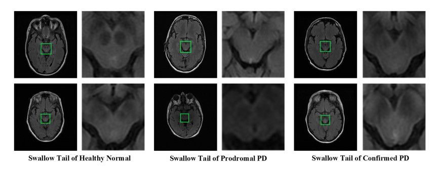
[28]	N. Wang, H. Yang, C. Li, G. Fan, X. Luo, Using 'swallow-tail' sign and putaminal hypointensity as biomarkers to distinguish multiple system atrophy from idiopathic Parkinson's disease: A susceptibility-weighted imaging study, Eur. Radiol., 27 (2017), 3174-3180. doi: 10.1007/s00330-017-4743-x
[29]	K. Machhale, H. B. Nandpuru, V Kapuret, L. Kosta, MRI brain cancer classification using hybrid classifier (SVM-KNN), 2015 International Conference on Industrial Instrumentation and Control (ICIC), 2015, 60-65. Available from: https://ieeexplore.ieee.org/abstract/document/7150592.
[30]	P. Refaeilzadeh, L. Tang, H. Liu, Cross-validation, E. Database Sys., 5 (2009), 532-538.
[31]	M. Kirby, Geometric data analysis: An empirical approach to dimensionality reduction and the study of patterns, John Wiley Sons, Inc., New York, NY, USA, 2001.
[32]	K. Honda, H. Ichihashi, Fuzzy local independent component analysis with external criteria and its application to knowledge discovery in databases, Int. J. Approximate Reasoning, 42 (2006), 159-173. doi: 10.1016/j.ijar.2005.10.011
[33]	D. Donoho, V. Stodden, When does non-negative matrix factorization give a correct decomposition into parts?, Proceedings of the 16^th International Conference on Neural Information Processing Systems, 2003, 1141-1148. Available from: http://papers.nips.cc/paper/2463-when-does-non-negative-matrix-factorization-give-a-correct-decomposition-into-parts.pdf.
[34]	A. Tharwat, Principal component analysis-a tutorial, Inderscience Enterprises Ltd, 3 (2016), 197-240.
[35]	T. Hastie, R. Tibshirani, Discriminant analysis by Gaussian mixtures, J. R. Stat. Soc. Series B, 58 (1996), 155-176.
[36]	G. E. Hinton, R. R. Salakhutdinov, Reducing the dimensionality of data with neural networks, Science, 313 (2006), 504-507. doi: 10.1126/science.1127647
[37]	S. Mika, G. Ratsch, J. Weston, B. Scholkopf, K. R. Mullers, Fisher discriminant analysis with kernels, Proceedings of the 1999 IEEE Signal Processing Society Workshop, Madison, 1999, 41-48. Available from: https://ieeexplore.ieee.org/abstract/document/788121.
[38]	Y. Yang, H. Wang, Multi-view clustering: A survey, Big Data Mining Anal., 1 (2018), 83-107. doi: 10.26599/BDMA.2018.9020003
[39]	U. Maulik, S. Bandyopadhyay, Performance evaluation of some clustering algorithms and validity indices, IEEE Trans. Pattern Anal. Mach. Intell., 24 (2002), 1650-1654. doi: 10.1109/TPAMI.2002.1114856

Reader Comments

Your name:*

Email:*
© 2020 the Author(s), licensee AIMS Press. This is an open access article distributed under the terms of the Creative Commons Attribution License (http://creativecommons.org/licenses/by/4.0)