A novel approach to modelling the spatial spread of airborne diseases: an epidemic model with indirect transmission

Jummy F. David; Sarafa A. Iyaniwura; Michael J. Ward; Fred Brauer; Jummy F. David; Sarafa A. Iyaniwura; Michael J. Ward; Fred Brauer

doi:10.3934/mbe.2020188

Mathematical Biosciences and Engineering

2020, Volume 17, Issue 4: 3294-3328. doi: 10.3934/mbe.2020188

Previous Article Next Article

Research article

A novel approach to modelling the spatial spread of airborne diseases: an epidemic model with indirect transmission

1.
Department of Mathematics, University of British Columbia, Vancouver, B.C., Canada
2.
Interdisciplinary Studies, University of British Columbia, Vancouver, B.C., Canada

Received: 03 December 2019 Accepted: 20 April 2020 Published: 27 April 2020

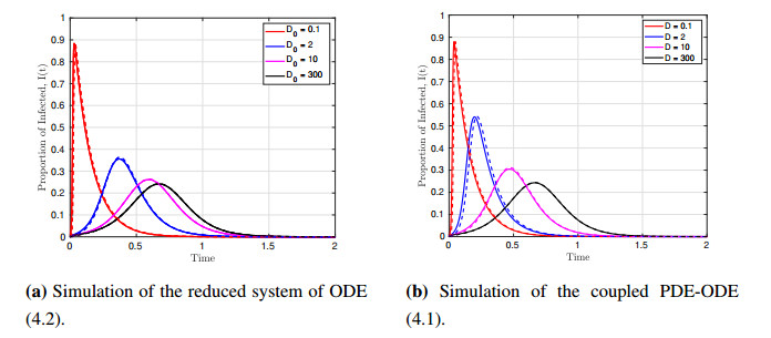
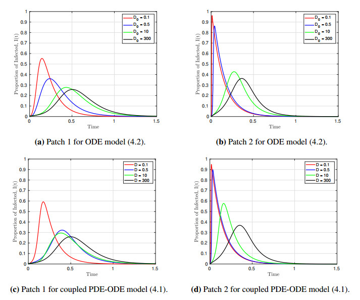
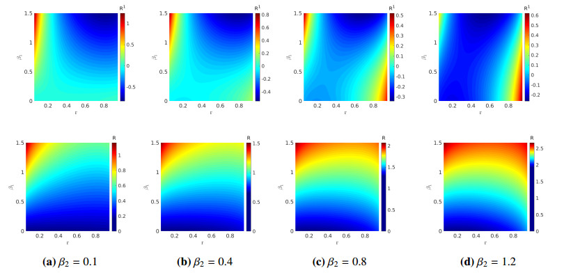
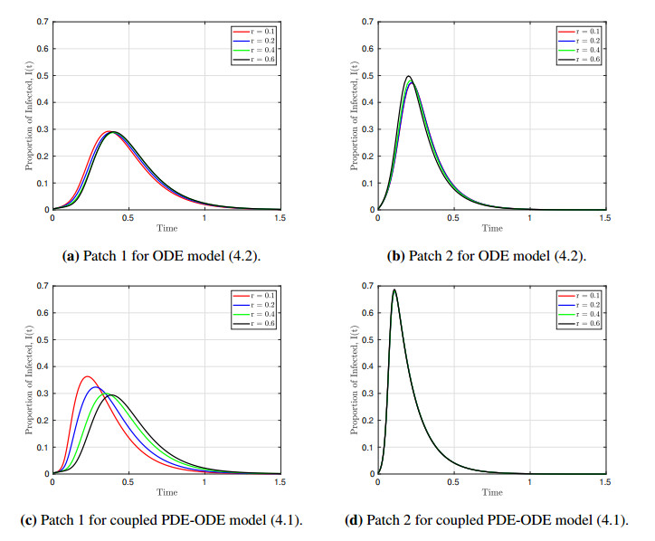
We formulated and analyzed a class of coupled partial and ordinary differential equation (PDE-ODE) model to study the spread of airborne diseases. Our model describes human populations with patches and the movement of pathogens in the air with linear diffusion. The diffusing pathogens are coupled to the SIR dynamics of each population patch using an integro-differential equation. Susceptible individuals become infected at some rate whenever they are in contact with pathogens (indirect transmission), and the spread of infection in each patch depends on the density of pathogens around the patch. In the limit where the pathogens are diffusing fast, a matched asymptotic analysis is used to reduce the coupled PDE-ODE model into a nonlinear system of ODEs, which is then used to compute the basic reproduction number and final size relation for different scenarios. Numerical simulations of the reduced system of ODEs and the full PDE-ODE model are consistent, and they predict a decrease in the spread of infection as the diffusion rate of pathogens increases. Furthermore, we studied the effect of patch location on the spread of infections for the case of two population patches. Our model predicts higher infections when the patches are closer to each other.
- disease dynamics,
- epidemics,
- airborne disease,
- indirect transmission,
- matched asymptotic analysis,
- Greenos function,
- ODE,
- PDE
Citation: Jummy F. David, Sarafa A. Iyaniwura, Michael J. Ward, Fred Brauer. A novel approach to modelling the spatial spread of airborne diseases: an epidemic model with indirect transmission[J]. Mathematical Biosciences and Engineering, 2020, 17(4): 3294-3328. doi: 10.3934/mbe.2020188

Related Papers:

Abstract

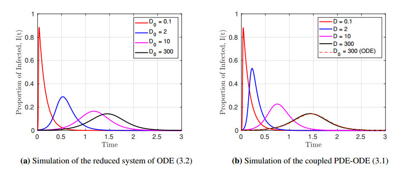
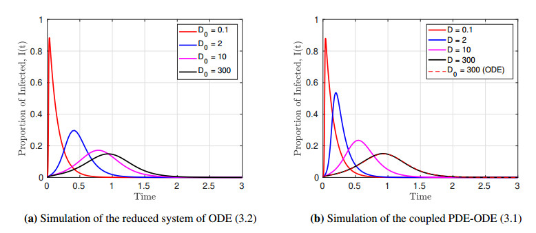
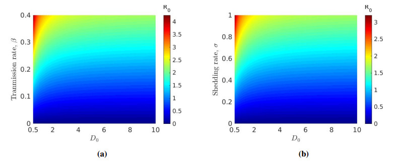
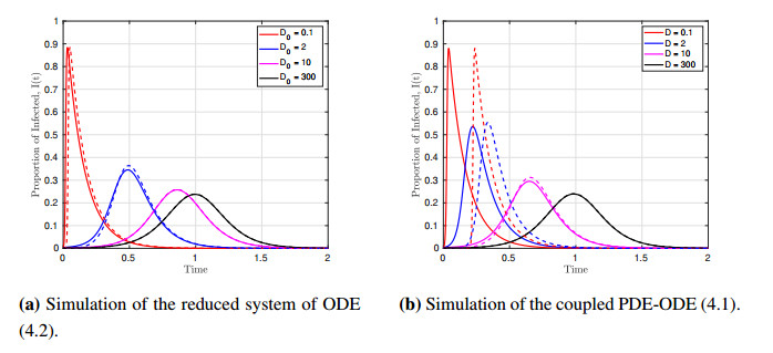
We formulated and analyzed a class of coupled partial and ordinary differential equation (PDE-ODE) model to study the spread of airborne diseases. Our model describes human populations with patches and the movement of pathogens in the air with linear diffusion. The diffusing pathogens are coupled to the SIR dynamics of each population patch using an integro-differential equation. Susceptible individuals become infected at some rate whenever they are in contact with pathogens (indirect transmission), and the spread of infection in each patch depends on the density of pathogens around the patch. In the limit where the pathogens are diffusing fast, a matched asymptotic analysis is used to reduce the coupled PDE-ODE model into a nonlinear system of ODEs, which is then used to compute the basic reproduction number and final size relation for different scenarios. Numerical simulations of the reduced system of ODEs and the full PDE-ODE model are consistent, and they predict a decrease in the spread of infection as the diffusion rate of pathogens increases. Furthermore, we studied the effect of patch location on the spread of infections for the case of two population patches. Our model predicts higher infections when the patches are closer to each other.

References

[1]	C. J. Noakes, C. B. Beggs, P. A. Sleigh, K. G. Kerr, Modelling the transmission of airborne infections in enclosed spaces, Epidemiol. Infect., 134 (2006), 1082-1091. doi: 10.1017/S0950268806005875
[2]	C. B. Beggs, The airborne transmission of infection in hospital buildings: Fact or fiction? Indoor Built Environ., 12 (2003), 9-18. doi: 10.1177/1420326X03012001002
[3]	C. M. Issarow, N. Mulder, R. Wood, Modelling the risk of airborne infectious disease using exhaled air. J. Theor. Biol., 372 (2015), 100-106. doi: 10.1016/j.jtbi.2015.02.010
[4]	Z. Xu, D. Chen, An SIS epidemic model with diffusion, Appl. Math. Ser. B, 32 (2017), 127-146. doi: 10.1007/s11766-017-3460-1
[5]	J. Ge, K. Kim, Z. Lin, H. Zhu, A SIS reaction-diffusion-advection model in a low-risk and high-risk domain, J. Differ. Equ., 259 (2015), 5486-5509. doi: 10.1016/j.jde.2015.06.035
[6]	M. Liu, Y. Xiao, Modeling and analysis of epidemic diffusion with population migration, J. Appl. Math., 2013 (2003), 583648.
[7]	N. Ziyadi, S. Boulite, M. L. Hbid, S. Touzeau, Mathematical analysis of a PDE epidemiological model applied to scrapie transmission, Commun. Pure Appl. Anal., 7 (2008), 659. doi: 10.3934/cpaa.2008.7.659
[8]	J. Gou, M. J. Ward, An asymptotic analysis of a 2-D model of dynamically active compartments coupled by bulk diffusion, J. Nonlinear Sci., 26 (2016), 979-1029. doi: 10.1007/s00332-016-9296-7
[9]	F. Brauer, A new epidemic model with indirect transmission, J. Biol. Dyn., 11 (2017), 285-293. doi: 10.1080/17513758.2016.1207813
[10]	J. F. David, Epidemic models with heterogeneous mixing and indirect transmission, J. Biol. Dyn., 12 (2018), 375-399. doi: 10.1080/17513758.2018.1467506
[11]	M. J. Ward, J. B. Keller, Strong localized perturbations of eigenvalue problems, SIAM J. Appl. Math., 53 (1993), 770-798. doi: 10.1137/0153038
[12]	PDE solutions Inc, FlexPDE 6, 2019.
[13]	F. Brauer, C. Castillo-Chavez, Mathematical Models in Population Biology and Epidemiology, 40, Springer, 2001.
[14]	O. Diekmann, J. A. P. Heesterbeek, J. A. J. Metz, On the definition and the computation of the basic reproduction ratio R 0 in models for infectious diseases in heterogeneous populations, J. Math. Biol., 28 (1990), 365-382.
[15]	P. V. den Driessche, J. Watmough, Reproduction numbers and sub-threshold endemic equilibria for compartmental models of disease transmission, Math. Biosci., 180 (2002), 29-48. doi: 10.1016/S0025-5564(02)00108-6
[16]	D. Bichara, Y. Kang, C. Castillo-Chavez, R. Horan, C. Perrings, SIS and SIR epidemic models under virtual dispersal, Bull. Math. Biol., 77 (2015), 2004-2034. doi: 10.1007/s11538-015-0113-5
[17]	F. Brauer, Epidemic models with heterogeneous mixing and treatment, Bull. Math. Biol., 70 (2008), 1869-1885. doi: 10.1007/s11538-008-9326-1
[18]	J. Arino, F. Brauer, P. Van Den Driessche, J. Watmough, J. Wu, A final size relation for epidemic models, Math. Biosci. Eng., 4 (2007), 159-175. doi: 10.3934/mbe.2007.4.159
[19]	F. Brauer, Age-of-infection and the final size relation, Math. Biosci. Eng., 5 (2008), 681-690. doi: 10.3934/mbe.2008.5.681
[20]	F. Brauer, The final size of a serious epidemic, Bull. Math. Biol., 81 (2019), 869-877. doi: 10.1007/s11538-018-00549-x
[21]	F. Brauer, A final size relation for epidemic models of vector-transmitted diseases, Infect. Dis. Model., 2 (2017), 12-20.
[22]	F. Brauer, C. Castillo-Chaavez, Mathematical models for communicable diseases, volume 84. SIAM, 2012.
[23]	F. Brauer, C. Castillo-Chavez, Z. Feng, Mathematical models in epidemiology, 2018.
[24]	L. F. Shampine, M. W. Reichelt, The Matlab ODE suite, SIAM J. Sci. Comput., 18 (1997), 1-22. doi: 10.1137/S1064827594276424
[25]	L. Zhang, Z.-C. Wang, Y. Zhang, Dynamics of a reaction-diffusion waterborne pathogen model with direct and indirect transmission, Comput. Math. Appl., 72 (2016), 202-215. doi: 10.1016/j.camwa.2016.04.046
[26]	T. Kolokolnikov, M. S. Titcombe, M. J. Ward, Optimizing the fundamental Neumann eigenvalue for the Laplacian in a domain with small traps, Europ. J. Appl. Math., 16 (2005), 161-200. doi: 10.1017/S0956792505006145
[27]	S. Chinviriyasit, W. Chinviriyasit, Numerical modelling of an SIR epidemic model with diffusion, Appl. Math. Comput., 216 (2010), 395-409.
[28]	H. Huang, M. Wang, The reaction-diffusion system for an SIR epidemic model with a free boundary, Discrete Cont. Dyn-B, 20 (2015), 2039-3050.
[29]	K. Ik Kim, Z. Lin, Asymptotic behavior of an SEI epidemic model with diffusion, Math. Comput. Model., 47 (2008), 1314-1322. doi: 10.1016/j.mcm.2007.08.004
[30]	E. M. Lotfi, M. Maziane, K. Hattaf, N. Yousfi, Partial differential equations of an epidemic model with spatial diffusion, Int. J. Part. Differ. Eq., 2014 (2014), 186437.
[31]	F. A. Milner, R. Zhao, Analysis of an SIR model with directed spatial diffusion, Math. Popul. Stud., 15 (2008), 160-181. doi: 10.1080/08898480802221889

Reader Comments

Your name:*

Email:*
© 2020 the Author(s), licensee AIMS Press. This is an open access article distributed under the terms of the Creative Commons Attribution License (http://creativecommons.org/licenses/by/4.0)