Coexistence and extinction in a data-based ratio-dependent model of an insect community

Yang Kuang; Kaifa Wang; Yang Kuang; Kaifa Wang

doi:10.3934/mbe.2020187

Mathematical Biosciences and Engineering

2020, Volume 17, Issue 4: 3274-3293. doi: 10.3934/mbe.2020187

Previous Article Next Article

Research article

Coexistence and extinction in a data-based ratio-dependent model of an insect community

Yang Kuang ^{1
,
,},
Kaifa Wang ^{2
,
,}

1.
School of Mathematical and Statistical Sciences, Arizona State University, Tempe, AZ 85287, USA
2.
School of Mathematics and Statistics, Southwest University, Chongqing 400715, P.R. China

Received: 24 February 2020 Accepted: 23 April 2020 Published: 27 April 2020

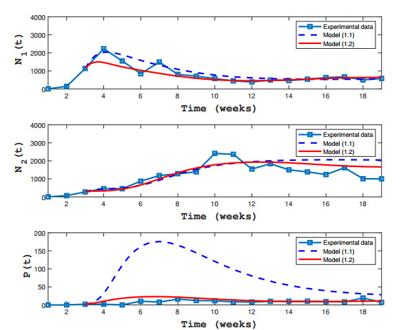
In theory, pure competition often leads to competitive exclusion of species. However, what we often see in nature is a large number of distinct predator or consumer species coexist in a community consisting a smaller number of prey or plant species. In an effort of dissecting how indirect competition and selective predation may have contributed to the coexistence of species in an insect community, according to the replicated cage experiments (two aphid species and a specialist parasitoid that attacks only one of the aphids) and proposed mathematical models, van Veen et. al. ^[5] conclude that the coexistence of the three species is due to a combination of density-mediated and trait-mediated indirect interactions. In this paper, we formulate an alternative model that observes the conventional law of mass conservation and provides a better fitting to their experimental data sets. Moreover, we present an initial attempt in studying the stabilities of the nonnegative steady states of this model.
- coexistence,
- extinction,
- competition,
- stability,
- Predator-prey,
- Hopf bifurcation
Citation: Yang Kuang, Kaifa Wang. Coexistence and extinction in a data-based ratio-dependent model of an insect community[J]. Mathematical Biosciences and Engineering, 2020, 17(4): 3274-3293. doi: 10.3934/mbe.2020187

Related Papers:

Abstract

In theory, pure competition often leads to competitive exclusion of species. However, what we often see in nature is a large number of distinct predator or consumer species coexist in a community consisting a smaller number of prey or plant species. In an effort of dissecting how indirect competition and selective predation may have contributed to the coexistence of species in an insect community, according to the replicated cage experiments (two aphid species and a specialist parasitoid that attacks only one of the aphids) and proposed mathematical models, van Veen et. al. ^[5] conclude that the coexistence of the three species is due to a combination of density-mediated and trait-mediated indirect interactions. In this paper, we formulate an alternative model that observes the conventional law of mass conservation and provides a better fitting to their experimental data sets. Moreover, we present an initial attempt in studying the stabilities of the nonnegative steady states of this model.

References

[1]	H. I. Freedman, Deterministic Mathematical Models in Population Ecology, Marcel Dekker, Inc., New York, (1980).
[2]	G. Hardin, The competitive exclusion principle, Science, 131 (1960), 1292-1297. doi: 10.1126/science.131.3409.1292
[3]	G. F. Gause, The Struggle For Existence, Baltimore, Williams & Wilkins, (1934).
[4]	Y. Kuang, H. I. Freedman, Uniqueness of limit cycles in Gause-type models of predator-prey systems, Math. Biosci., 88 (1988), 67-84. doi: 10.1016/0025-5564(88)90049-1
[5]	F. J. F. van Veen, P. D. van Holland, H. C. J. Godfray, Stable coexistence in insect communities due to density- and trait-mediated indirect effects, Ecology, 86 (2005), 3182-3189. doi: 10.1890/04-1590
[6]	S. B. Hsu, T. W. Hwang, Y. Kuang, Rich dynamics of a ratio-dependent one prey two predator model, J. Math. Biol., 43 (2001), 377-396. doi: 10.1007/s002850100100
[7]	S. B. Hsu, T. W. Hwang, Y. Kuang, A ratio-dependent food chain model and its applications to biological control, Math. Biosci., 181 (2003), 55-83. doi: 10.1016/S0025-5564(02)00127-X
[8]	Y. Kuang, E. Beretta, Global qualitative analysis of a ratio-dependent predator-prey system, J. Math. Biol., 36 (1998), 389-406. doi: 10.1007/s002850050105
[9]	S. B. Hsu, T. W. Hwang, Y. Kuang, Global analysis of the Michaelis-Menten-type ratio-dependent predator-prey system, J. Math. Biol., 42 (2001), 489-506. doi: 10.1007/s002850100079
[10]	T. W. Hwang, Y. Kuang, Deterministic extinction effect of parasites on host populations, J. Math. Biol., 46 (2003), 17-30. doi: 10.1007/s00285-002-0165-7
[11]	T. W. Hwang, Y. Kuang, Host extinction dynamics in a simple parasite-host interaction model, Math. Biosci. Eng., 2 (2005), 743-751. doi: 10.3934/mbe.2005.2.743
[12]	P. Waltman, A Second Course in Elementary Differential Equations, Reprinted, Dover Publications, (2004).
[13]	E. Beretta, Y. Kuang, Modeling and analysis of a marine bacteriophage infection, Math. Biosci., 149 (1998), 57-76. doi: 10.1016/S0025-5564(97)10015-3
[14]	Z. E. Ma, Mathematical modeling and research of population ecology, Hefei: Anhui Education Press, (1996).
[15]	Y. Kuang, J. D. Nagy, S. E. Eikenberry, Introduction to mathematical oncology, Chapman and HallCRC, (2016).
[16]	W. M. Liu, Criterion of Hopf bifurcations without using eigenvalues, J. Math. Anal. Appl., 182 (1994), 250-256. doi: 10.1006/jmaa.1994.1079
[17]	S. Hews, S. Eikenberry, J. D. Nagy, Y. Kuang, Rich dynamics of a hepatitis B viral infection model with logistic hepatocyte growth, J. Math. Biol., 60 (2010), 573-590. doi: 10.1007/s00285-009-0278-3
[18]	H. R. Thieme, Mathematics in population biology, Princeton, (2003).
[19]	E. Beretta, Y. Kuang, Modeling and analysis of a marine bacteriophage infection with latency period, Nonlinear Anal. RWA, 2 (2001), 35-74. doi: 10.1016/S0362-546X(99)00285-0
[20]	E. Beretta, Y. Kuang, Geometric stability switch criteria in delay differential systems with delay dependent parameters, SIAM J. Math. Anal., 33 (2002), 1144-1165. doi: 10.1137/S0036141000376086
[21]	S. A. Gourley, Y. Kuang, A stage structured predator-prey model and its dependence on maturation delay and death rate, J. Math. Biol., 49 (2004), 188-200.
[22]	Y. Kuang, Delay differential equations with applications in population dynamics, Academic Press, (1993).
[23]	E. Beretta, Y. Kuang, Global analyses in some delayed ratio-dependent predator-prey systems, Nonlinear Anal. TMA, 32 (1998), 381-408. doi: 10.1016/S0362-546X(97)00491-4
[24]	Y. Kuang, W. Fagan, I. Loladze, Biodiversity, habitat area, resource growth rate and interference competition, Bull. Math. Biol., 65 (2003), 497-518. doi: 10.1016/S0092-8240(03)00008-9
[25]	R. Sterner, J. J. Elser, Ecological Stoichiometry, Princeton University Press, Princeton, NJ, (2002).
[26]	I. Loladze, Y. Kuang, J. J. Elser, Stoichiometry in producer-grazer systems: linking energy flow and element cycling, Bull. Math. Biol., 62 (2000), 1137-1162. doi: 10.1006/bulm.2000.0201
[27]	I. Loladze, Y. Kuang, J. J. Elser, W. F. Fagan, Coexistence of two predators on one prey mediated by stoichiometry, Theor. Popul. Biol., 65 (2004), 1-15. doi: 10.1016/S0040-5809(03)00105-9
[28]	X. Yang, X. Li, H. Wang, Y. Kuang, Stability and bifurcation in a stoichiometric producer-grazer model with knife edge, SIAM J. Appl. Dyn. Syst., 15 (2016), 2051-2077. doi: 10.1137/15M1023610
[29]	M. Chen, M. Fan, Y. Kuang, Global dynamics in a stoichiometric food chain model with two limiting nutrients, Math. Biosci., 289 (2017), 9-19. doi: 10.1016/j.mbs.2017.04.004
[30]	J. J. Elser, I. Loladze, A. L. Peace, Y. Kuang, Lotka re-loaded: Modeling trophic interactions under stoichiometric constraints, Ecol. Model., 245 (2012), 3-11. doi: 10.1016/j.ecolmodel.2012.02.006
[31]	A. Peace, H. Wang, Y. Kuang, Dynamics of a producer-grazer model incorporating the effects of excess food-nutrient content on grazer's growth, Bull. Math. Biol., 76 (2014), 2175-2197. doi: 10.1007/s11538-014-0006-z
[32]	J. J. Elser, Y. Kuang, Ecological stoichiometry. In: Hastings, A., Gross, L. (eds.), Encyclopedia of Theoretical Ecology, University of California Press, (2012), 718-722.
[33]	D. O. Hessen, J. J. Elser, R. W. Sterner, J. Urabe, Ecological stoichiometry: An elementary approach using basic principles, Limnol. Oceanogr., 58 (2013), 2219-2236. doi: 10.4319/lo.2013.58.6.2219

Reader Comments

Your name:*

Email:*
© 2020 the Author(s), licensee AIMS Press. This is an open access article distributed under the terms of the Creative Commons Attribution License (http://creativecommons.org/licenses/by/4.0)