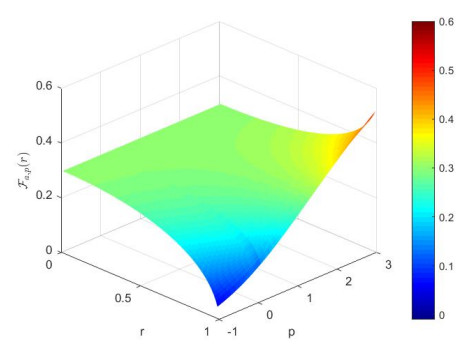
This paper deals with the second kind of generalized elliptic integral $\mathcal{E}_a$, for $a$ in the interval $\left[\frac{1}{2}, 1\right)$, approximated by the weighted Hölder mean. It establishes sharp bounds of the weighted Hölder mean of $\mathcal{E}_a$ in terms of weight, accordingly extending the existing results for the complete case when $ a = \frac{1}{2} $ and establishing new inequality relationships.
Citation: Zixuan Wang, Chuanlong Sun, Tiren Huang. Sharp weighted Hölder mean bounds for the second kind generalized elliptic integral[J]. AIMS Mathematics, 2025, 10(5): 11271-11289. doi: 10.3934/math.2025511
This paper deals with the second kind of generalized elliptic integral $\mathcal{E}_a$, for $a$ in the interval $\left[\frac{1}{2}, 1\right)$, approximated by the weighted Hölder mean. It establishes sharp bounds of the weighted Hölder mean of $\mathcal{E}_a$ in terms of weight, accordingly extending the existing results for the complete case when $ a = \frac{1}{2} $ and establishing new inequality relationships.

| [1] | M. Abramowitz, I. A. Stegun, D. Miller, Handbook of mathematical functions with formulas, graphs, and mathematical tables (National Bureau of Standards Applied Mathematics Series No. 55), J. Appl. Mech., 32 (1965), 239. https://doi.org/10.1115/1.3625776 |
| [2] | J. M. Borwein, P. B. Borwein, Pi and the AGM, John Wiley & Sons, 1987. |
| [3] | G. D. Anderson, M. K. Vamanamurthy, M. Vuorinen, Conformal invariants, inequalities, and quasiconformal maps, John Wiley & Sons, 1997. |
| [4] | S. L. Qiu, M. K. Vamanamurthy, M. Vuorinen, Some inequalities for the Hersch-Pfluger distortion function, J. Inequal. Appl., 4 (1999), 115–139. https://doi.org/10.1155/S1025583499000326 |
| [5] | G. D. Anderson, S. L. Qiu, M. K. Vamanamurthy, M. Vuorinen, Generalized elliptic integrals and modular equations, Pacific J. Math., 192 (2000), 1–37. https://doi.org/10.2140/pjm.2000.192.1 |
| [6] |
H. Alzer, K. Richards, On the modulus of the Grötzsch ring, J. Math. Anal. Appl., 432 (2015), 134–141. https://doi.org/10.1016/j.jmaa.2015.06.057 doi: 10.1016/j.jmaa.2015.06.057

|
| [7] |
W. M. Qian, Z. Y. He, Y. M. Chu, Approximation for the complete elliptic integral of the first kind, RACSAM, 114 (2020), 57. https://doi.org/10.1007/s13398-020-00784-9 doi: 10.1007/s13398-020-00784-9
|
| [8] |
J. F. Tian, Z. H. Yang, M. H. Ha, H. J. Xing, A family of high order approximations of Ramanujan type for perimeter of an ellipse, RACSAM, 115 (2021), 85. https://doi.org/10.1007/s13398-021-01021-7 doi: 10.1007/s13398-021-01021-7
|
| [9] |
T. H. Zhao, M. K. Wang, Discrete approximation of complete $p$-elliptic integral of the second kind and its application, RACSAM, 118 (2024), 37. https://doi.org/10.1007/s13398-023-01537-0 doi: 10.1007/s13398-023-01537-0
|
| [10] |
M. K. Wang, H. H. Chu, Y. M. Chu, Precise bounds for the weighted Hölder mean of the complete $p$-elliptic integrals, J. Math. Anal. Appl., 480 (2019), 123388. https://doi.org/10.1016/j.jmaa.2019.123388 doi: 10.1016/j.jmaa.2019.123388
|
| [11] |
Z. H. Yang, J. F. Tian, Sharp bounds for the Toader mean in terms of arithmetic and geometric means, RACSAM, 115 (2021), 99. https://doi.org/10.1007/s13398-021-01040-4 doi: 10.1007/s13398-021-01040-4
|
| [12] | R. W. Barnard, K. Pearce, K. C. Richards, An inequality involving the generalized hypergeometric function and the arc length of an ellipse, SIAM J. Math. Anal., 31 (2000), 693–699. https://doi.org/10.1137/S0036141098341575 |
| [13] | H. Alzer, S. L. Qiu, Monotonicity theorems and inequalities for the complete elliptic integrals, J. Comput. Appl. Math., 172 (2004), 289–312. https://doi.org/10.1016/j.cam.2004.02.009 |
| [14] | P. S. Bullen, Handbook of means and their inequalities, Springer Science & Business Media, 2003. |
| [15] | M. K. Wang, Z. Y. He, T. H. Zhao, Q. Bao, Sharp weighted Hölder mean bounds for the complete elliptic integral of the second kind, Integr. Transf. Spec. Funct., 34 (2023), 537–551. https://doi.org/10.1080/10652469.2022.2155819 |
| [16] |
V. Heikkala, M. K. Vamanamurthy, M. Vuorinen, Generalized elliptic integrals, Comput. Methods Funct. Theory, 9 (2009), 75–109. https://doi.org/10.1007/BF03321716 doi: 10.1007/BF03321716
|
| [17] |
Q. I. Rahman, On the monotonicity of certain functionals in the theory of analytic functions, Can. Math. Bull., 10 (1967), 723–729. https://doi.org/10.4153/CMB-1967-074-9 doi: 10.4153/CMB-1967-074-9
|
| [18] | Z. H. Yang, Recurrence relations of coefficients involving hypergeometric function with an application, arXiv, 2022. https://doi.org/10.48550/arXiv.2204.04709 |


Figures(3)

Zixuan Wang, Chuanlong Sun, Tiren Huang. Sharp weighted Hölder mean bounds for the second kind generalized elliptic integral[J]. AIMS Mathematics, 2025, 10(5): 11271-11289. doi: 10.3934/math.2025511


 DownLoad: