In this paper, a new hybrid meta-heuristic algorithm called CEBWO (cross-entropy method and beluga whale optimization) is presented to solve the mean-CVaR portfolio optimization problem based on jump-diffusion processes. The proposed CEBWO algorithm combines the advantages of the cross-entropy method and beluga whale optimization algorithm with the help of co-evolution technology to enhance the performance of portfolio selection. The method is evaluated on 29 unconstrained benchmark functions from CEC 2017, where its performance is compared against several state-of-the-art algorithms. The results demonstrate the superiority of the hybrid method in terms of solution quality and convergence speed. Finally, Monte Carlo simulation is employed to generate scenario paths based on the jump-diffusion model. Empirical results further confirm the effectiveness of the hybrid meta-heuristic algorithm for mean-CVaR portfolio selection, highlighting its potential for real-world applications.
Citation: Guocheng Li, Pan Zhao, Minghua Shi, Gensheng Li. A hybrid framework for mean-CVaR portfolio selection under jump-diffusion processes: Combining cross-entropy method with beluga whale optimization[J]. AIMS Mathematics, 2024, 9(8): 19911-19942. doi: 10.3934/math.2024972
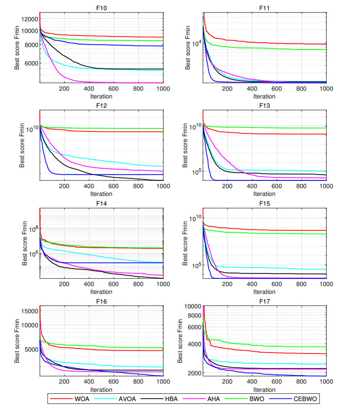
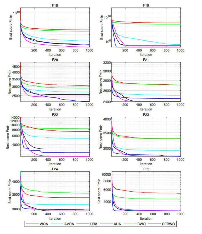
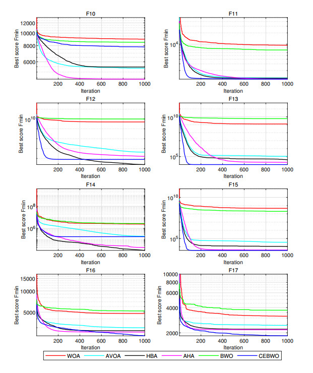
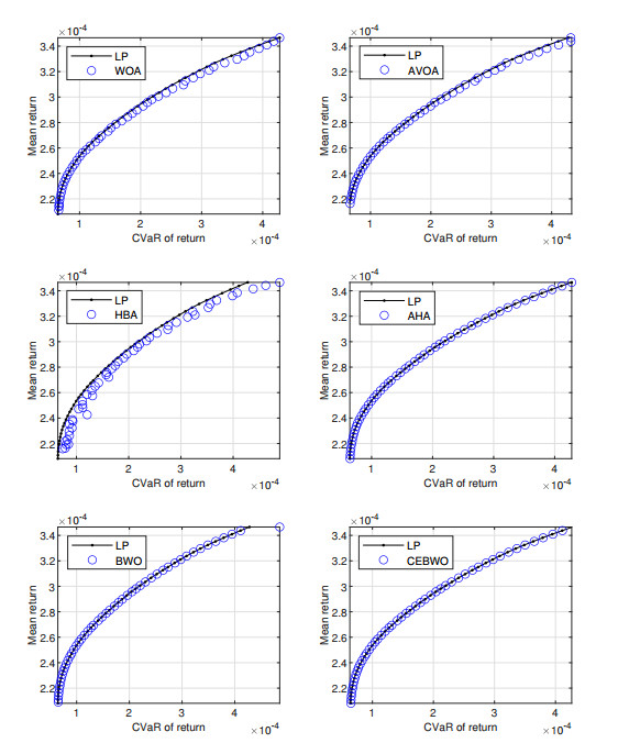
In this paper, a new hybrid meta-heuristic algorithm called CEBWO (cross-entropy method and beluga whale optimization) is presented to solve the mean-CVaR portfolio optimization problem based on jump-diffusion processes. The proposed CEBWO algorithm combines the advantages of the cross-entropy method and beluga whale optimization algorithm with the help of co-evolution technology to enhance the performance of portfolio selection. The method is evaluated on 29 unconstrained benchmark functions from CEC 2017, where its performance is compared against several state-of-the-art algorithms. The results demonstrate the superiority of the hybrid method in terms of solution quality and convergence speed. Finally, Monte Carlo simulation is employed to generate scenario paths based on the jump-diffusion model. Empirical results further confirm the effectiveness of the hybrid meta-heuristic algorithm for mean-CVaR portfolio selection, highlighting its potential for real-world applications.

| [1] |
H. Markowitz, Portfolio selection, J. Fin., 7 (1952), 77–91. https://doi.org/10.2307/2975974 doi: 10.2307/2975974

|
| [2] |
P. Artzner, F. Delbaen, J. Eber, D. Heath, Coherent measures of risk, Math. Financ., 9 (1999), 203–228. https://doi.org/10.1111/1467-9965.00068 doi: 10.1111/1467-9965.00068
|
| [3] | J. Longerstaey, M. Spencer, Riskmetricstm–Technical document, 4 Eds., New York: Morgan Guaranty Trust Company of New York, 1996. |
| [4] |
F. Y. Chen, Analytical VaR for international portfolios with common jumps, Comput. Math. Appl., 62 (2011), 3066–3076. https://doi.org/10.1016/j.camwa.2011.08.018 doi: 10.1016/j.camwa.2011.08.018
|
| [5] |
J. W. Goh, K. G. Lim, M. Sim, W. Zhang, Portfolio value-at-risk optimization for asymmetrically distributed asset returns, Eur. J. Oper. Res., 221 (2012), 397–406. https://doi.org/10.1016/j.ejor.2012.03.012 doi: 10.1016/j.ejor.2012.03.012
|
| [6] |
S. Basak, A. Shapiro, Value-at-risk based risk management: Optimal policies and asset prices, Rev. Fin. Stud., 14 (2001), 371–405. https://doi.org/10.1093/rfs/14.2.371 doi: 10.1093/rfs/14.2.371
|
| [7] |
T. Rockfeller, S. Uryasev, Optimization of conditional value-at-risk, J. Risk, 2 (2000), 21–41. https://doi.org/10.21314/JOR.2000.038 doi: 10.21314/JOR.2000.038
|
| [8] |
R. T. Rockfeller, S. Uryasev, Conditional value-at-risk for general loss distribution, J. Bank. Financ., 26 (2002), 1443–1471. https://doi.org/10.1016/S0378-4266(02)00271-6 doi: 10.1016/S0378-4266(02)00271-6
|
| [9] |
S. Alexander, T. F. Coleman, Y. Li, Minimizing CVaR and VaR for a portfolio of derivatives, J. Bank. Finan., 30 (2006), 583–605. https://doi.org/10.1016/j.jbankfin.2005.04.012 doi: 10.1016/j.jbankfin.2005.04.012
|
| [10] |
S. Zhu, M. Fukushima, Worst-case conditional value-at-risk with application to robust portfolio management, Oper. Res., 57 (2009), 1155–1168. https://doi.org/10.1287/opre.1080.0684 doi: 10.1287/opre.1080.0684
|
| [11] |
S. Yau, R. H. Kwon, J. S. Rogers, D. Wu, Financial and operational decisions in the electricity sector: Contract portfolio optimization with the conditional value-at-risk criterion, Int. J. Prod. Econ., 134 (2011), 67–77. https://doi.org/10.1016/j.ijpe.2010.10.007 doi: 10.1016/j.ijpe.2010.10.007
|
| [12] |
L. J. Hong, G. Liu, Simulating sensitivities of conditional value at risk, Manage. Sci., 55 (2009), 281–293. https://doi.org/10.1287/mnsc.1080.0901 doi: 10.1287/mnsc.1080.0901
|
| [13] |
S. Zhao, Q. Lu, L. Han, Y. Liu, F. Hu, A mean-CVaR-skewness portfolio optimization model based on asymmetric Laplace distribution, Ann. Oper. Res., 226 (2015), 727–739. https://doi.org/10.1007/s10479-014-1654-y doi: 10.1007/s10479-014-1654-y
|
| [14] |
F. G. Ferreira, R. T. Cardoso, Mean-CVaR portfolio optimization approaches with variable cardinality constraint and rebalancing process, Arch. Comput. Method. Eng., 28 (2021), 3703–3720. https://doi.org/10.1007/s11831-020-09522-1 doi: 10.1007/s11831-020-09522-1
|
| [15] |
C. I. Fábián, Handling CVaR objectives and constraints in two-stage stochastic models, Eur. J. Oper. Res., 191 (2008), 888–911. https://doi.org/10.1016/j.ejor.2007.02.052 doi: 10.1016/j.ejor.2007.02.052
|
| [16] |
W. Liu, L. Yang, B. Yu, Kernel density estimation based distributionally robust mean-CVaR portfolio optimization, J. Glob. Optim., 84 (2022), 1053–1077. https://doi.org/10.1007/s10898-022-01177-5 doi: 10.1007/s10898-022-01177-5
|
| [17] |
N. Abudurexiti, K. He, D. Hu, S. T. Rachev, H. Sayit, R. Sun, Portfolio analysis with mean-CVaR and mean-CVaR-skewness criteria based on mean–variance mixture models, Ann. Oper. Res., 336 (2024), 945–966. https://doi.org/10.1007/s10479-023-05396-1 doi: 10.1007/s10479-023-05396-1
|
| [18] |
F. Q. Lu, M. Huang, W. K. Ching, T. K. Siu, Credit portfolio management using two-level particle swarm optimization, Inform. Sci., 237 (2013), 162–175. https://doi.org/10.1016/j.ins.2013.03.005 doi: 10.1016/j.ins.2013.03.005
|
| [19] |
T. Zhang, Z. Liu, Fireworks algorithm for mean-VaR/CVaR models, Physica A: Stat. Mech. Appl., 483 (2017), 1–8. https://doi.org/10.1016/j.physa.2017.04.036 doi: 10.1016/j.physa.2017.04.036
|
| [20] |
J. Zhai, M. Bai, H. Wu, Mean-risk-skewness models for portfolio optimization based on uncertain measure, Optimization, 67 (2018), 701–714. https://doi.org/10.1080/02331934.2018.1426577 doi: 10.1080/02331934.2018.1426577
|
| [21] |
Y. Li, B. Zhou, Y. Tan, Portfolio optimization model with uncertain returns based on prospect theory, Complex Intell. Syst., 8 (2022), 4529–4542. https://doi.org/10.1007/s40747-021-00493-9 doi: 10.1007/s40747-021-00493-9
|
| [22] |
F. Lu, T. Yan, H. Bi, M. Feng, S. Wang, M. Huang, A bilevel whale optimization algorithm for risk management scheduling of information technology projects considering outsourcing, Knowl.-Based Syst., 235 (2022), 107600. https://doi.org/10.1016/j.knosys.2021.107600 doi: 10.1016/j.knosys.2021.107600
|
| [23] |
J. Danane, M. Yavuz, M. Yıldız, Stochastic modeling of three-species prey–predator model driven by Lévy Jump with Mixed Holling-Ⅱ and Beddington–DeAngelis functional responses, Fractal Fract., 7 (2023), 751. https://doi.org/10.3390/fractalfract7100751 doi: 10.3390/fractalfract7100751
|
| [24] |
Y. Song, G. Zhao, B. Zhang, H. Chen, W. Deng, W. Deng, An enhanced distributed differential evolution algorithm for portfolio optimization problems, Eng. Appl. Artif. Intel., 121 (2023), 106004. https://doi.org/10.1016/j.engappai.2023.106004 doi: 10.1016/j.engappai.2023.106004
|
| [25] |
X. S. Yang, A. H. Gandomi, Bat algorithm: A novel approach for global engineering optimization, Eng. Computation., 29 (2012), 464–483. https://doi.org/10.1108/02644401211235834 doi: 10.1108/02644401211235834
|
| [26] |
A. H. Gandomi, A. H. Alavi, Krill herd: A new bio-inspired optimization algorithm, Commun. Nonlinear Sci., 12 (2012), 4831–4845. https://doi.org/ 10.1016/j.cnsns.2012.05.010 doi: 10.1016/j.cnsns.2012.05.010
|
| [27] |
S. Mirjalili, S. M. Mirjalili, A. Lewis, Grey wolf optimizer, Adv. Eng. Softw., 69 (2014), 46–61. https://doi.org/10.1016/j.advengsoft.2013.12.007 doi: 10.1016/j.advengsoft.2013.12.007
|
| [28] |
A. Askarzadeh, A novel metaheuristic method for solving constrained engineering optimization problems: Crow search algorithm, Comput. Struct., 169 (2016), 1–12. https://doi.org/10.1016/j.compstruc.2016.03.001 doi: 10.1016/j.compstruc.2016.03.001
|
| [29] |
S. Mirjalili, A. Lewis, The whale optimization algorithm, Adv. Eng. Softw., 95 (2016), 51–67. https://doi.org/10.1016/j.advengsoft.2016.01.008 doi: 10.1016/j.advengsoft.2016.01.008
|
| [30] |
S. Saremi, S. Mirjalili, A. Lewis, Grasshopper optimisation algorithm: Theory and application, Adv. Eng. Softw., 105 (2017), 30–47. https://doi.org/10.1016/j.advengsoft.2017.01.004 doi: 10.1016/j.advengsoft.2017.01.004
|
| [31] |
G. Wang, Moth search algorithm: A bio-inspired metaheuristic algorithm for global optimization problems, Memetic Comp., 10 (2018), 151–164. https://doi.org/10.1007/s12293-016-0212-3 doi: 10.1007/s12293-016-0212-3
|
| [32] |
N. A. Kallioras, N. D. Lagaros, D. N. Avtzis, Pity beetle algorithm–A new metaheuristic inspired by the behavior of bark beetles, Adv. Eng. Softw., 147 (2018), 147–166. https://doi.org/10.1016/j.advengsoft.2018.04.007 doi: 10.1016/j.advengsoft.2018.04.007
|
| [33] |
A. A. Heidari, S. Mirjalili, H. Faris, I. Aljarah, M. Mafarja, H. Chen, Harris hawks optimization: Algorithm and applications, Future Gener. Comp. Syst., 97 (2019), 849–872. https://doi.org/10.1016/j.future.2019.02.028 doi: 10.1016/j.future.2019.02.028
|
| [34] |
M. Jain, V. Singh, A. Rani, A novel nature-inspired algorithm for optimization: Squirrel search algorithm, Swarm Evol. Comput., 44 (2019), 148–175. https://doi.org/10.1016/j.swevo.2018.02.013 doi: 10.1016/j.swevo.2018.02.013
|
| [35] |
S. Arora, S. Singh, Butterfly optimization algorithm: A novel approach for global optimization, Soft Comput., 23 (2019), 715–734. https://doi.org/10.1007/s00500-018-3102-4 doi: 10.1007/s00500-018-3102-4
|
| [36] |
A. Faramarzi, M. Heidarinejad, S. Mirjalili, A. H. Gandomi, Marine Predators Algorithm: A nature-inspired metaheuristic, Expert Syst. Appl., 152 (2020), 113377. https://doi.org/10.1016/j.eswa.2020.113377 doi: 10.1016/j.eswa.2020.113377
|
| [37] |
M. Khishe, M. R. Mosavi, Chimp optimization algorithm, Expert Syst. Appl., 149 (2020), 113338. https://doi.org/10.1016/j.eswa.2020.113338 doi: 10.1016/j.eswa.2020.113338
|
| [38] |
S. Li, H. Chen, M. Wang, A. A. Heidari, S. Mirjalili, Slime mould algorithm: A new method for stochastic optimization, Future Gener. Comp. Syst., 111 (2020), 300–323. https://doi.org/10.1016/j.future.2020.03.055 doi: 10.1016/j.future.2020.03.055
|
| [39] |
A. Mohammadi-Balani, M. D. Nayeri, A. Azar, M. Taghizadeh-Yazdi, Golden eagle optimizer: A nature-inspired metaheuristic algorithm, Comput. Ind. Eng., 152 (2021), 107050. https://doi.org/10.1016/j.cie.2020.107050 doi: 10.1016/j.cie.2020.107050
|
| [40] |
D. Połap, M. Woźniak, Red fox optimization algorithm, Expert Syst. Appl., 166 (2021), 114107. https://doi.org/10.1016/j.eswa.2020.114107 doi: 10.1016/j.eswa.2020.114107
|
| [41] |
Y. Yang, H. Chen, A. A. Heidari, A. H. Gandomi, Hunger games search: Visions, conception, implementation, deep analysis, perspectives, and towards performance shifts, Expert Syst. Appl., 177 (2021), 114864. https://doi.org/10.1016/j.eswa.2021.114864 doi: 10.1016/j.eswa.2021.114864
|
| [42] |
I. Ahmadianfar, A. A. Heidari, A. H. Gandomi, X. Chu, H. Chen, RUN beyond the metaphor: An efficient optimization algorithm based on Runge Kutta method, Expert Syst. Appl., 181 (2021), 115079. https://doi.org/10.1016/j.eswa.2021.115079 doi: 10.1016/j.eswa.2021.115079
|
| [43] |
J. Tu, H. Chen, M. Wang, A. H. Gandomi, The colony predation algorithm, J. Bionic Eng., 181 (2021), 674–710. https://doi.org/10.1007/s42235-021-0050-y doi: 10.1007/s42235-021-0050-y
|
| [44] |
I. Ahmadianfar, A. A. Heidari, S. Noshadian, H. Chen, A. H Gandomi, INFO: An efficient optimization algorithm based on weighted mean of vectors, Expert Syst. Appl., 195 (2021), 116516. https://doi.org/10.1016/j.eswa.2022.116516 doi: 10.1016/j.eswa.2022.116516
|
| [45] |
B. Abdollahzadeh, F. S. Gharehchopogh, S. Mirjalili, African vultures optimization algorithm: A new nature-inspired metaheuristic algorithm for global optimization problems, Comput. Ind. Eng., 158 (2021), 107408. https://doi.org/10.1016/j.cie.2021.107408 doi: 10.1016/j.cie.2021.107408
|
| [46] |
B. Abdollahzadeh, F. S. Gharehchopogh, S. Mirjalili, Artificial gorilla troops optimizer: A new nature-inspired metaheuristic algorithm for global optimization problems, Int. J. Intell. Syst., 36 (2021), 5887–5958. https://doi.org/10.1002/int.22535 doi: 10.1002/int.22535
|
| [47] |
F. A. Hashim, E. H. Houssein, K. Hussain, M. S. Mabrouk, W. Al-Atabany, Honey Badger Algorithm: New metaheuristic algorithm for solving optimization problems, Math. Comput. Simulat., 192 (2022), 84–110. https://doi.org/10.1016/j.matcom.2021.08.013 doi: 10.1016/j.matcom.2021.08.013
|
| [48] |
W. Zhao, L. Wang, S. Mirjalili, Artificial hummingbird algorithm: A new bio-inspired optimizer with its engineering applications, Comput. Method. Appl. Mech. Eng., 388 (2022), 114194. https://doi.org/10.1016/j.cma.2021.114194 doi: 10.1016/j.cma.2021.114194
|
| [49] |
B. Abdollahzadeh, F. S. Gharehchopogh, N. Khodadadi, S. Mirjalili, Mountain gazelle optimizer: A new nature-inspired metaheuristic algorithm for global optimization problems, Adv. Eng. Softw., 174 (2022), 103282. https://doi.org/10.1016/j.advengsoft.2022.103282 doi: 10.1016/j.advengsoft.2022.103282
|
| [50] |
E. H. Houssein, D. Oliva, N. A. Samee, N. F. Mahmoud, M. M. Emam, Liver Cancer Algorithm: A novel bio-inspired optimizer, Comput. Biol. Med., 165 (2023), 107389. https://doi.org/10.1016/j.compbiomed.2023.107389 doi: 10.1016/j.compbiomed.2023.107389
|
| [51] |
H. Su, D. Zhao, A. A. Heidari, L. Liu, X. Zhang, M. Mafarja, et al., RIME: A physics-based optimization, Neurocomputing, 532 (2023), 183–214. https://doi.org/10.1016/j.neucom.2023.02.010 doi: 10.1016/j.neucom.2023.02.010
|
| [52] |
C. Zhong, G. Li, Z. Meng, Beluga whale optimization: A novel nature-inspired metaheuristic algorithm, Knowl.-Based Syst., 251 (2022), 109215. https://doi.org/10.1016/j.knosys.2022.109215 doi: 10.1016/j.knosys.2022.109215
|
| [53] |
D. H. Wolpert, W. G. Macready, No free lunch theorems for optimization, IEEE T. Evolut. Comput., 1 (1997), 67–82. https://doi.org/10.1109/4235.585893 doi: 10.1109/4235.585893
|
| [54] |
M. M. Mafarja, S. Mirjalili, Hybrid whale optimization algorithm with simulated annealing for feature selection, Neurocomputing, 260 (2017), 302–312. https://doi.org/10.1016/j.neucom.2017.04.053 doi: 10.1016/j.neucom.2017.04.053
|
| [55] |
M. Abdel-Basset, W. Ding, D. El-Shahat, A hybrid Harris Hawks optimization algorithm with simulated annealing for feature selection, Artif Intell. Rev., 54 (2021), 593–637. https://doi.org/10.1007/s10462-020-09860-3 doi: 10.1007/s10462-020-09860-3
|
| [56] |
P. J. Gaidhane, M. J. Nigam, A hybrid grey wolf optimizer and artificial bee colony algorithm for enhancing the performance of complex systems, J. Comput. Sci., 27 (2018), 284–302. https://doi.org/10.1016/j.jocs.2018.06.008 doi: 10.1016/j.jocs.2018.06.008
|
| [57] |
B. Farnad, A. Jafarian, D. Baleanu, A new hybrid algorithm for continuous optimization problem, Appl. Math. Model., 55 (2018), 652–673. https://doi.org/10.1016/j.apm.2017.10.001 doi: 10.1016/j.apm.2017.10.001
|
| [58] |
M. AkbaiZadeh, T. Niknam, A. Kavousi-Fard, Adaptive robust optimization for the energy management of the grid-connected energy hubs based on hybrid meta-heuristic algorithm, Energy, 235 (2021), 121171. https://doi.org/10.1016/j.energy.2021.121171 doi: 10.1016/j.energy.2021.121171
|
| [59] |
A. A. Najafi, S. Mushakhian, Multi-stage stochastic mean–semivariance–CVaR portfolio optimization under transaction costs, Appl. Math. Comput., 256 (2015), 445–458. https://doi.org/10.1016/j.amc.2015.01.050 doi: 10.1016/j.amc.2015.01.050
|
| [60] |
M. F. Leung, J. Wang, Cardinality-constrained portfolio selection based on collaborative neurodynamic optimization, Neural Networks, 145 (2022), 68–79. https://doi.org/10.1016/j.neunet.2021.10.007 doi: 10.1016/j.neunet.2021.10.007
|
| [61] |
H. Sorensen, Parametric inference for diffusion processes observed at discrete points in time: A survey, Int. Stat. Rev., 72 (2004), 337–354. https://doi.org/10.1111/j.1751-5823.2004.tb00241.x doi: 10.1111/j.1751-5823.2004.tb00241.x
|
| [62] | R. Cont, P. Tankov, Financial modelling with jump processes, 1 Eds., New York: Chapman and Hall/CRC, 2003. https://doi.org/10.1201/9780203485217 |
| [63] |
D. Ardia, J. David, O. Arango, N. D. G. Gómez, Jump-diffusion calibration using differential evolution, Wilmott, 55 (2011), 76–79. https://doi.org/10.1002/wilm.10034 doi: 10.1002/wilm.10034
|
| [64] |
R. Y. Rubinstein, Optimization of computer simulation models with rare events, Eur. J. Oper. Res., 99 (1997), 89–112. https://doi.org/10.1016/S0377-2217(96)00385-2 doi: 10.1016/S0377-2217(96)00385-2
|
| [65] |
P. T. de Boer, D. P. Kroese, R. Y. Rubinstein, A fast cross-entropy method for estimating buffer overflows in queueing networks, Manage. Sci., 50 (2004), 883–895. https://doi.org/10.1287/mnsc.1030.0139 doi: 10.1287/mnsc.1030.0139
|
| [66] |
J. C. Chan, D. P. Kroese, Improved cross-entropy method for estimation, Stat. Comput., 22 (2012), 1031–1040. https://doi.org/10.1007/s11222-011-9275-7 doi: 10.1007/s11222-011-9275-7
|
| [67] |
G. Alon, D. P. Kroese, T. Raviv, R. Y. Rubinstein, Application of the cross-entropy method to the buffer allocation problem in a simulation-based environment, Ann. Oper. Res., 134 (2005), 137–151. https://doi.org/10.1007/s10479-005-5728-8 doi: 10.1007/s10479-005-5728-8
|
| [68] |
R. Caballero, A. G. Hernández-Díaz, M. Laguna, J. Molina, Cross entropy for multiobjective combinatorial optimization problems with linear relaxations, Eur. J. Oper. Res., 243 (2015), 362–368. https://doi.org/10.1016/j.ejor.2014.07.046 doi: 10.1016/j.ejor.2014.07.046
|
| [69] |
R. Rubinstein, The cross-entropy method for combinatorial and continuous optimization, Methodol. Comput. Appl., 1 (1999), 127–190. https://doi.org/10.1023/A:1010091220143 doi: 10.1023/A:1010091220143
|
| [70] |
D. P. Kroese, S. Porotsky, R. Y. Rubinstein, The cross-entropy method for continuous multi-extremal optimization, Methodol. Comput. Appl., 8 (2006), 383–407. https://doi.org/10.1007/s11009-006-9753-0 doi: 10.1007/s11009-006-9753-0
|
| [71] |
J. Bekker, C. Aldrich, The cross-entropy method in multi-objective optimisation: An assessment, Eur. J. Oper. Res., 211 (2011), 112–121. https://doi.org/10.1016/j.ejor.2010.10.028 doi: 10.1016/j.ejor.2010.10.028
|
| [72] |
K. Chepuri, T. Homem-De-Mello, Solving the vehicle routing problem with stochastic demands using the cross-entropy method, Ann. Oper. Res., 134 (2005), 153–181. https://doi.org/10.1007/s10479-005-5729-7 doi: 10.1007/s10479-005-5729-7
|
| [73] |
I. Szita, A. Lörincz, Learning Tetris using the noisy cross-entropy method, Neural Comput., 18 (2006), 2936–2941. https://doi.org/10.1162/neco.2006.18.12.2936 doi: 10.1162/neco.2006.18.12.2936
|
| [74] |
M. Laguna, A. Duarte, R. Marti, Hybridizing the cross-entropy method: An application to the max-cut problem, Comput. Oper. Res., 36 (2009), 487–498. https://doi.org/10.1016/j.cor.2007.10.001 doi: 10.1016/j.cor.2007.10.001
|
| [75] |
M. Maher, R. Liu, D. Ngoduy, Signal optimization using the cross entropy method, Transport. Res. C: Emer. Technol., 27 (2013), 76–88. https://doi.org/10.1016/j.trc.2011.05.018 doi: 10.1016/j.trc.2011.05.018
|
| [76] |
G. R. Lamonica, M. C. Recchioni, F. M. Chelli, L. Salvati, The efficiency of the cross-entropy method when estimating the technical coefficients of input-output tables, Spat. Econ. Anal., 15 (2020), 62–91. https://doi.org/10.1080/17421772.2019.1615634 doi: 10.1080/17421772.2019.1615634
|
| [77] |
M. L. Cardoso, L. F. Venturini, Y. L. Baracy, I. M. B. Ulisses, L. E. Bremermann, A. P. Grilo-Pavani, et al., Fault indicator placement optimization using the cross-entropy method and traffic simulation data, Electr. Pow. Syst. Res., 212 (2022), 108391. https://doi.org/10.1016/j.epsr.2022.108391 doi: 10.1016/j.epsr.2022.108391
|
| [78] |
A. E. Eiben, C. A. Schipper, On evolutionary exploration and exploitation, Fund. Inform., 35 (1998), 35–50. https://doi.org/10.3233/FI-1998-35123403 doi: 10.3233/FI-1998-35123403
|
| [79] |
H. Chen, Z. Wang, D. Wu, H. Jia, C. Wen, H. Rao, et al., An improved multi-strategy beluga whale optimization for global optimization problems, Math. Biosci. Eng., 20 (2023), 13267–13317. https://doi.org/10.3934/mbe.2023592 doi: 10.3934/mbe.2023592
|
| [80] |
A. G. Hussien, R. A. Khurma, A. Alzaqebah, M. Amin, F. A. Hashim, Novel memetic of beluga whale optimization with self-adaptive exploration–exploitation balance for global optimization and engineering problems, Soft Comput., 27 (2023), 13951–13989. https://doi.org/10.1007/s00500-023-08468-3 doi: 10.1007/s00500-023-08468-3
|
| [81] | N. H. Awad, M. Z. Ali, P. N. Suganthan, J. J. Liang, B. Y. Qu, Problem defnitions and evaluation criteria for the CEC 2017 special session and competition on single objective real-parameter numerical optimization, 2016. Available from: https://github.com/P-N-Suganthan/CEC2017-BoundContrained/blob/master/Definitions%20of%20%20CEC2017%20benchmark%20suite%20final%20version%20updated.pdf. |
| [82] | P. Fortune, Are stock returns different over weekends? A jump diffusion analysis of the weekend effect, In: New England Economic Review, 10 (1999), 3–19. https://fedinprint.org/item/fedbne/41360 |
Figures(9) / Tables(5)

Guocheng Li, Pan Zhao, Minghua Shi, Gensheng Li. A hybrid framework for mean-CVaR portfolio selection under jump-diffusion processes: Combining cross-entropy method with beluga whale optimization[J]. AIMS Mathematics, 2024, 9(8): 19911-19942. doi: 10.3934/math.2024972


 DownLoad: