Analytical and numerical investigation of viscous fluid-filled spherical slip cavity in a spherical micropolar droplet

Abdulaziz H. Alharbi; Ahmed G. Salem; Abdulaziz H. Alharbi; Ahmed G. Salem

doi:10.3934/math.2024732

AIMS Mathematics

2024, Volume 9, Issue 6: 15097-15118. doi: 10.3934/math.2024732

Previous Article Next Article

Research article Special Issues

Analytical and numerical investigation of viscous fluid-filled spherical slip cavity in a spherical micropolar droplet

Abdulaziz H. Alharbi ^{1
,
,},
Ahmed G. Salem ^{2
,
,}

1.
Department of Mathematics, Jamoum University College, Umm Al-Qura University, Jamoum, 25375, Makkah, Saudi Arabia
2.
Department of Mathematics, Faculty of Science, Mansoura University, 35516, Mansoura, Egypt

Received: 20 February 2024 Revised: 23 March 2024 Accepted: 19 April 2024 Published: 26 April 2024
MSC : 35Q30, 76B99, 76D05, 76T06

This article presents an analytical and numerical investigation on the quasi-steady, slow flow generated by the movement of a micropolar fluid drop sphere of at a concentrical position within another immiscible viscous fluid inside a spherical slip cavity. Additionally, the effect of a cavity with slip friction along with the change in the micropolarity parameter on the movement of the fluid sphere is introduced. When Reynolds numbers are low, the droplet moves along a diameter that connects their centres. The governing and constitutive differential equations are reduced to a computationally convenient form using appropriate transformations. By using the resulting linear partial differential equations for the stream functions and using the method of separation variables, we can obtain their solutions. General solutions for velocity fields are found using spherical coordinate systems, which are based on the concentric point of the cavity; this allows to obtain solutions to the Navier-Stokes equations internal and external to the spherical droplet. The vorticity-microrotation boundary condition is used in regard to the micropolar droplet case in a viscous fluid. The normalised drag forces acted upon the micropolar drop are illustrated via graphs and tables for diverse values of the viscosity ratio and drop-to-wall radius ratio, with the change of the spin parameter that attaches the microrotation to vorticity. The correction wall factor is shown to increase with an increase in the drop-to-wall radius ratio, when moving from the gas bubble case to the solid sphere case, with an increase in the micropolarity parameter, and with an increase in the slip frictional resistance. This study is relevant due to its potential uses in a variety of biological, natural, and industrial processes, including the creation of raindrops, the investigation of blood flow, fluid-fluid extraction, the forecasting of weather conditions, the rheology of emulsions, and sedimentation phenomena.
- low Reynolds numbers,
- micropolar fluid,
- vorticity-microrotation condition,
- spherical slip cavity
Citation: Abdulaziz H. Alharbi, Ahmed G. Salem. Analytical and numerical investigation of viscous fluid-filled spherical slip cavity in a spherical micropolar droplet[J]. AIMS Mathematics, 2024, 9(6): 15097-15118. doi: 10.3934/math.2024732

Related Papers:

Abstract

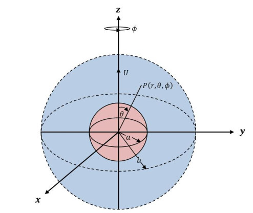
This article presents an analytical and numerical investigation on the quasi-steady, slow flow generated by the movement of a micropolar fluid drop sphere of at a concentrical position within another immiscible viscous fluid inside a spherical slip cavity. Additionally, the effect of a cavity with slip friction along with the change in the micropolarity parameter on the movement of the fluid sphere is introduced. When Reynolds numbers are low, the droplet moves along a diameter that connects their centres. The governing and constitutive differential equations are reduced to a computationally convenient form using appropriate transformations. By using the resulting linear partial differential equations for the stream functions and using the method of separation variables, we can obtain their solutions. General solutions for velocity fields are found using spherical coordinate systems, which are based on the concentric point of the cavity; this allows to obtain solutions to the Navier-Stokes equations internal and external to the spherical droplet. The vorticity-microrotation boundary condition is used in regard to the micropolar droplet case in a viscous fluid. The normalised drag forces acted upon the micropolar drop are illustrated via graphs and tables for diverse values of the viscosity ratio and drop-to-wall radius ratio, with the change of the spin parameter that attaches the microrotation to vorticity. The correction wall factor is shown to increase with an increase in the drop-to-wall radius ratio, when moving from the gas bubble case to the solid sphere case, with an increase in the micropolarity parameter, and with an increase in the slip frictional resistance. This study is relevant due to its potential uses in a variety of biological, natural, and industrial processes, including the creation of raindrops, the investigation of blood flow, fluid-fluid extraction, the forecasting of weather conditions, the rheology of emulsions, and sedimentation phenomena.

References

[1]	S. S. Sadhal, P. S. Ayyaswamy, J. N. Chung, Transport phenomena with drops and bubbles, Springer Science & Business Media, 2012. https://doi.org/10.1007/978-1-4612-4022-8
[2]	U. Ali, K. U. Rehman, A. S. Alshomrani, M. Y. Malik, Thermal and concentration aspects in Carreau viscosity model via wedge, Case Stud. Therm. Eng., 12 (2018), 126–133. https://doi.org/10.1016/j.csite.2018.04.007 doi: 10.1016/j.csite.2018.04.007
[3]	M. Waqas, Z. Asghar, W. A. Khan, Thermo-solutal Robin conditions significance in thermally radiative nanofluid under stratification and magnetohydrodynamics, Eur. Phys. J. Spec. Top., 230 (2021), 1307–1316. https://doi.org/10.1140/epjs/s11734-021-00044-w doi: 10.1140/epjs/s11734-021-00044-w
[4]	K. U. Rehman, W. Shatanawi, Q. M. Al-Mdallal, A comparative remark on heat transfer in thermally stratified MHD Jeffrey fluid flow with thermal radiations subject to cylindrical/plane surfaces, Case Stud. Therm. Eng., 32 (2022), 101913. https://doi.org/10.1016/j.csite.2022.101913 doi: 10.1016/j.csite.2022.101913
[5]	T. Kebede, E. Haile, G. Awgichew, T. Walelign, Heat and mass transfer in unsteady boundary layer flow of Williamson nanofluids, J. Appl. Math., 2020 (2020), 1–13. https://doi.org/10.1155/2020/1890972 doi: 10.1155/2020/1890972
[6]	T. Walelign, E. Haile, T. Kebede, G. Awgichew, Heat and mass transfer in stagnation point flow of Maxwell nanofluid towards a vertical stretching sheet with effect of induced magnetic field, Math. Probl. Eng., 2021 (2021), 1–15. https://doi.org/10.1155/2021/6610099 doi: 10.1155/2021/6610099
[7]	G. G. Stokes, On the effect of the internal friction of fluids on the motion of pendulums, T. Cambridge Philos. Soc., 3 (1851), 8–106.
[8]	W. Rybczynski, Über die fortschreitende Bewegung einer flussigen Kugel in einem zahen Medium, Bull. Acad. Sci. Cracovie A, 1 (1911), 40–46.
[9]	M. J. Hadamard, Mécanique-mouvement permanent lent d'une sphèere liquide et visqueuse dans un liquid visqueux, Compt. Rend. Acad. Sci., 152 (1911), 1735–1738.
[10]	R. Niefer, P. N. Kaloni, On the motion of a micropolar fluid drop in a viscous fluid, J. Eng. Math., 14 (1980), 107–116. https://doi.org/10.1007/BF00037621 doi: 10.1007/BF00037621
[11]	T. D. Taylor, A. Acrivos, On the deformation and drag of a falling viscous drop at low Reynolds number, J. Fluid Mech., 18 (1964), 466–476. https://doi.org/10.1017/S0022112064000349 doi: 10.1017/S0022112064000349
[12]	E. Bart, The slow unsteady settling of a fluid sphere toward a flat fluid interface, Chem. Eng. Sci., 23 (1968), 193–210. https://doi.org/10.1016/0009-2509(86)85144-2 doi: 10.1016/0009-2509(86)85144-2
[13]	G. Hetsroni, S. Haber, E. Wacholder, The flow fields in and around a droplet moving axially within a tube, J. Fluid Mech., 41 (1970), 689–705. https://doi.org/10.1017/S0022112070000848 doi: 10.1017/S0022112070000848
[14]	H. Brenner, Pressure drop due to the motion of neutrally buoyant particles in duct flows. Ⅱ. Spherical droplets and bubbles, Ind. Eng. Chem. Fund., 10 (1971), 537–543. https://doi.org/10.1021/i160040a001 doi: 10.1021/i160040a001
[15]	E. Wacholder, D. Weihs, Slow motion of a fluid sphere in the vicinity of another sphere or a plane boundary, Chem. Eng. Sci., 27 (1972), 1817–1828. https://doi.org/10.1016/0009-2509(72)85043-7 doi: 10.1016/0009-2509(72)85043-7
[16]	E. Rushton, G. A. Davies, The slow unsteady settling of two fluid spheres along their line of centres, Appl. Sci. Res., 28 (1973), 37–61. https://doi.org/10.1007/BF00413056 doi: 10.1007/BF00413056
[17]	M. Coutanceau, P. Thizon, Wall effect on the bubble behaviour in highly viscous liquids, J. Fluid Mech., 107 (1981), 339–373. https://doi.org/10.1017/S0022112081001808 doi: 10.1017/S0022112081001808
[18]	M. Shapira, S. Haber, Low Reynolds number motion of a droplet between two parallel plates, Int. J. Multiphase Flow, 14 (1988), 483–506. https://doi.org/10.1016/0301-9322(88)90024-9 doi: 10.1016/0301-9322(88)90024-9
[19]	H. J. Keh, Y. K. Tseng, Slow motion of multiple droplets in arbitrary three-dimensional configurations, AICHE J., 38 (1992), 1881–1904. https://doi.org/10.1002/aic.690381205 doi: 10.1002/aic.690381205
[20]	H. J. Keh, P. Y. Chen, Slow motion of a droplet between two parallel plane walls, Chem. Eng. Sci., 56 (2001), 6863–6871. https://doi.org/10.1016/S0009-2509(01)00323-2 doi: 10.1016/S0009-2509(01)00323-2
[21]	J. Magnaudet, S. H. U. Takagi, L. Dominique, Drag, deformation and lateral migration of a buoyant drop moving near a wall, J. Fluid Mech., 476 (2003), 115–157. https://doi.org/10.1017/S0022112002002902 doi: 10.1017/S0022112002002902
[22]	A. Z. Zinchenko, R. H. Davis, A multipole-accelerated algorithm for close interaction of slightly deformable drops, J. Comput. Phys., 207 (2005), 695–735. https://doi.org/10.1016/j.jcp.2005.01.026 doi: 10.1016/j.jcp.2005.01.026
[23]	H. J. Keh, Y. C. Chang, Creeping motion of a slip spherical particle in a circular cylindrical pore, Int. J. Multiphase Flow, 33 (2007), 726–741. https://doi.org/10.1016/j.ijmultiphaseflow.2006.12.008 doi: 10.1016/j.ijmultiphaseflow.2006.12.008
[24]	C. Pozrikidis, Interception of two spherical drops in linear Stokes flow, J. Eng. Math., 66 (2010), 353–379. https://doi.org/10.1007/s10665-009-9301-3 doi: 10.1007/s10665-009-9301-3
[25]	K. Sugiyama, F. Takemura, On the lateral migration of a slightly deformed bubble rising near a vertical plane wall, J. Fluid Mech., 662 (2010), 209–231. https://doi.org/10.1017/S0022112010003149 doi: 10.1017/S0022112010003149
[26]	K. Sangtae, S. J. Karrila, Microhydrodynamics: Principles and selected applications, Courier Corporation, 2013.
[27]	T. C. Lee, H. J. Keh, Creeping motion of a fluid drop inside a spherical cavity, Eur. J. Mech. B-Fluid., 34 (2012), 97–104. https://doi.org/10.1016/j.euromechflu.2012.01.008 doi: 10.1016/j.euromechflu.2012.01.008
[28]	K. U. Rehman, A. S. Alshomrani, M. Y. Malik, Carreau fluid flow in a thermally stratified medium with heat generation/absorption effects, Case Stud. Therm. Eng., 12 (2018), 16–25. https://doi.org/10.1016/j.csite.2018.03.001 doi: 10.1016/j.csite.2018.03.001
[29]	Z. Asghar, M. W. S. Khan, M. A. Gondal, A. Ghaffari, Channel flow of non-Newtonian fluid due to peristalsis under external electric and magnetic field, Proc. I. Mech. Eng. Part E, 236 (2022), 2670–2678. https://doi.org/10.1177/09544089221097693 doi: 10.1177/09544089221097693
[30]	A. G. Salem, M. S. Faltas, H. H. Sherief, Migration of nondeformable droplets in a circular tube filled with micropolar fluids, Chinese J. Phys., 79 (2022), 287–305. https://doi.org/10.1016/j.cjph.2022.08.003 doi: 10.1016/j.cjph.2022.08.003
[31]	A. C. Eringen, Simple microfluids, Int. J. Eng. Sci., 2 (1964), 205–217. https://doi.org/10.1016/0020-7225(64)90005-9 doi: 10.1016/0020-7225(64)90005-9
[32]	A. C. Eringen, Theory of micropolar fluids, J. Math. Mech., 1966, 1–18. https://www.jstor.org/stable/24901466
[33]	V. K Stokes, Theories of fluids with microstructure, New York: Springer, 1984. https://doi.org/10.1007/978-3-642-82351-0_4
[34]	G. A. Graham, Continuum mechanics and its applications, Hemisphere Publishing Corporation, 1989,707–720.
[35]	H. Hayakawa, Slow viscous flows in micropolar fluids, Phys. Rev. E, 61 (2000), 5477. https://doi.org/10.1103/PhysRevE.61.5477 doi: 10.1103/PhysRevE.61.5477
[36]	T. Walelign, E. Seid, Mathematical model analysis for hydromagnetic flow of micropolar nanofluid with heat and mass transfer over inclined surface, Int. J. Thermofluids, 21 (2024), 100541. https://doi.org/10.1016/j.ijft.2023.100541 doi: 10.1016/j.ijft.2023.100541
[37]	E. H. Kennard, Kinetic theory of gases, 483 (1938), New York: McGraw-hill. https://doi.org/10.1038/142494a0
[38]	D. K. Hutchins, M. H. Harper, R. L. Felder, Slip correction measurements for solid spherical particles by modulated dynamic light scattering, Aerosol Sci. Tech., 22 (1995), 202–218. https://doi.org/10.1080/02786829408959741 doi: 10.1080/02786829408959741
[39]	P. A. Thompson, S. M. Troian, A general boundary condition for liquid flow at solid surfaces, Nature, 389 (1997), 360–362. https://doi.org/10.1038/38686 doi: 10.1038/38686
[40]	Z. Asghar, R. A. Shah, N. Ali, A computational approach to model gliding motion of an organism on a sticky slime layer over a solid substrate, Biomech. Model. Mechan., 21 (2022), 1441–1455. https://doi.org/10.1007/s10237-022-01600-6 doi: 10.1007/s10237-022-01600-6
[41]	E. Seid, E. Haile, T. Walelign, Multiple slip, Soret and Dufour effects in fluid flow near a vertical stretching sheet in the presence of magnetic nanoparticles, Int. J. Thermofluids, 13 (2022), 100136. https://doi.org/10.1016/j.ijft.2022.100136 doi: 10.1016/j.ijft.2022.100136
[42]	C. L. Navier, Mémoire sur les lois du mouvement des fluides, Mem. Acad. Roy. Sci. I. Fr., 6 (1823), 389–440.
[43]	J. L. Barrat, Large slip effect at a nonwetting fluid-solid interface, Phys. Rev. Lett., 82 (1999), 4671. https://doi.org/10.1103/PhysRevLett.82.4671 doi: 10.1103/PhysRevLett.82.4671
[44]	C. Neto, D. R. Evans, E. Bonaccurso, H. J. Butt, V. S. J. Craig, Boundary slip in Newtonian liquids: A review of experimental studies, Rep. Prog. Phys., 68 (2005), 2859. https://doi.org/10.1088/0034-4885/68/12/R05 doi: 10.1088/0034-4885/68/12/R05
[45]	W. Jäger, A. Mikelić, On the roughness-induced effective boundary conditions for an incompressible viscous flow, J. Differ. Equations, 170 (2001), 96–122. https://doi.org/10.1006/jdeq.2000.3814 doi: 10.1006/jdeq.2000.3814
[46]	D. C. Tretheway, C. D. Meinhart, Apparent fluid slip at hydrophobic microchannel walls, Phys. Fluids, 14 (2002), L9–L12. https://doi.org/10.1063/1.1432696 doi: 10.1063/1.1432696
[47]	G. Willmott, Dynamics of a sphere with inhomogeneous slip boundary conditions in Stokes flow, Phys. Rev. E, 77 (2008), 055302. https://doi.org/10.1103/PhysRevE.77.055302 doi: 10.1103/PhysRevE.77.055302
[48]	D. Bucur, E. Feireisl, Š. Nečasová, Influence of wall roughness on the slip behaviour of viscous fluids, P. Roy. Soc. Edinb. A, 138 (2008), 957–973. https://doi.org/10.1017/S0308210507000376 doi: 10.1017/S0308210507000376
[49]	F. Yang, Slip boundary condition for viscous flow over solid surfaces, Chem. Eng. Commun., 197 (2009), 544–550. https://doi.org/10.1080/00986440903245948 doi: 10.1080/00986440903245948
[50]	H. Sun, C. Liu, The slip boundary condition in the dynamics of solid particles immersed in Stokesian flows, Solid State Commun., 150 (2010), 990–1002. https://doi.org/10.1016/j.ssc.2010.01.017 doi: 10.1016/j.ssc.2010.01.017
[51]	H. Zhang, Z. Zhang, Y. Zheng, H. Ye, Corrected second-order slip boundary condition for fluid flows in nanochannels, Phys. Rev. E, 81 (2010), 066303. https://doi.org/10.1103/PhysRevE.81.066303 doi: 10.1103/PhysRevE.81.066303
[52]	K. H. Hoffmann, D. Marx, N. D. Botkin, Drag on spheres in micropolar fluids with non-zero boundary conditions for microrotations, J. Fluid Mech., 590 (2007), 319–330. https://doi.org/10.1017/S0022112007008099 doi: 10.1017/S0022112007008099
[53]	A. G. Salem, Effects of a spherical slip cavity filled with micropolar fluid on a spherical viscous droplet, Chinese J. Phys., 86 (2023), 98–114. https://doi.org/10.1016/j.cjph.2023.09.004 doi: 10.1016/j.cjph.2023.09.004
[54]	H. H. Sherif, M. S. Faltas, E. I. Saad, Slip at the surface of a sphere translating perpendicular to a plane wall in micropolar fluid, Z. Angew. Math. Phys., 59 (2008), 293–312. https://doi.org/10.1007/s00033-007-6078-y doi: 10.1007/s00033-007-6078-y
[55]	A. G. Salem, Effects of a spherical slip cavity filled with micropolar fluid on a spherical micropolar droplet, Fluid Dyn. Res., 55 (2023), 065502. https://doi.org/10.1088/1873-7005/ad0ee3 doi: 10.1088/1873-7005/ad0ee3
[56]	J. Happel, H. Brenner, Low Reynolds number hydrodynamics: With special applications to particulate media, Germany: Springer Netherlands, 2012. https://doi.org/10.1007/978-94-009-8352-6
[57]	A. C. Eringen, Microcontinuum field theories: II. Fluent media, 2 (2001), Springer Science & Business Media.
[58]	E. Cunningham, On the velocity of steady fall of spherical particles through fluid medium, Proc. Roy. Soc. London Ser. A, 83 (1910), 357–365. https://doi.org/10.1098/rspa.1910.0024 doi: 10.1098/rspa.1910.0024
[59]	W. L. Haberman, R. M. Sayre, Motion of rigid and fluid spheres in stationary and moving liquids inside cylindrical tubes, David Taylor Model Basin Washington DC, 1958. http://hdl.handle.net/1721.3/48988
[60]	N. P. Migun, On hydrodynamic boundary conditions for microstructural fluids, Rheol. Acta, 23 (1984), 575–581. https://doi.org/10.1007/BF01438797 doi: 10.1007/BF01438797
[61]	H. Ramkissoon, S. R. Majumdar, Drag on an axially symmetric body in the Stokes' flow of micropolar fluid, Phys. Fluids, 19 (1976), 16–21. https://doi.org/10.1063/1.861320 doi: 10.1063/1.861320

Reader Comments

Your name:*

Email:*
© 2024 the Author(s), licensee AIMS Press. This is an open access article distributed under the terms of the Creative Commons Attribution License (http://creativecommons.org/licenses/by/4.0)