The fractal-fractional Atangana-Baleanu operator for pneumonia disease: stability, statistical and numerical analyses

Najat Almutairi; Sayed Saber; Hijaz Ahmad; Najat Almutairi; Sayed Saber; Hijaz Ahmad

doi:10.3934/math.20231504

AIMS Mathematics

2023, Volume 8, Issue 12: 29382-29410. doi: 10.3934/math.20231504

Previous Article Next Article

Research article

The fractal-fractional Atangana-Baleanu operator for pneumonia disease: stability, statistical and numerical analyses

1.
Department of Mathematics, College of Science, Qassim University, Buraidah, Saudi Arabia
2.
Department of Mathematics and Statistics, Faculty of Science, Beni-Suef University, Egypt
3.
Department of Mathematics, Faculty of Science and Arts in Baljurashi, Al-Baha University, Saudi Arabia
4.
Near East University, Operational Research Center in Healthcare, Nicosia, Turkey
5.
Department of Computer Science and Mathematics, Lebanese American University, Beirut, Lebanon
6.
Section of Mathematics, International Telematic University Uninettuno, Corso Vittorio Emanuele Ⅱ, 39, 00186, Rome, Italy

Received: 03 September 2023 Revised: 02 October 2023 Accepted: 11 October 2023 Published: 30 October 2023
MSC : 34C60, 92B05, 92C42, 92D25, 92D30

The present paper studies pneumonia transmission dynamics by using fractal-fractional operators in the Atangana-Baleanu sense. Our model predicts pneumonia transmission dynamically. Our goal is to generalize five ODEs of the first order under the assumption of five unknowns (susceptible, vaccinated, carriers, infected, and recovered). The Atangana-Baleanu operator is used in addition to analysing existence, uniqueness, and non-negativity of solutions, local and global stability, Hyers-Ulam stability, and sensitivity analysis. As long as the basic reproduction number $ \mathscr{R}_{0} $ is less than one, the free equilibrium point is local, asymptotic, or otherwise global. Our sensitivity statistical analysis shows that $ \mathscr{R}_{0} $ is most sensitive to pneumonia disease density. Further, we compute a numerical solution for the model by using fractal-fractional. Graphs of the results are presented for demonstration of our proposed method. The results of the Atangana-Baleanu fractal-fractional scheme is in excellent agreement with the actual data.
- fractional derivatives,
- nonlinear equations,
- simulation,
- numerical results,
- infectious disease,
- time varying control system
Citation: Najat Almutairi, Sayed Saber, Hijaz Ahmad. The fractal-fractional Atangana-Baleanu operator for pneumonia disease: stability, statistical and numerical analyses[J]. AIMS Mathematics, 2023, 8(12): 29382-29410. doi: 10.3934/math.20231504

Related Papers:

Abstract

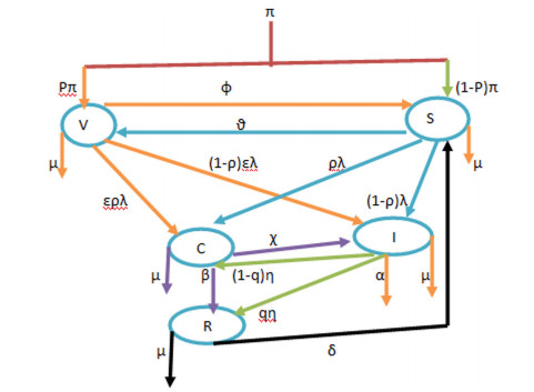
The present paper studies pneumonia transmission dynamics by using fractal-fractional operators in the Atangana-Baleanu sense. Our model predicts pneumonia transmission dynamically. Our goal is to generalize five ODEs of the first order under the assumption of five unknowns (susceptible, vaccinated, carriers, infected, and recovered). The Atangana-Baleanu operator is used in addition to analysing existence, uniqueness, and non-negativity of solutions, local and global stability, Hyers-Ulam stability, and sensitivity analysis. As long as the basic reproduction number $ \mathscr{R}_{0} $ is less than one, the free equilibrium point is local, asymptotic, or otherwise global. Our sensitivity statistical analysis shows that $ \mathscr{R}_{0} $ is most sensitive to pneumonia disease density. Further, we compute a numerical solution for the model by using fractal-fractional. Graphs of the results are presented for demonstration of our proposed method. The results of the Atangana-Baleanu fractal-fractional scheme is in excellent agreement with the actual data.

References

[1]	A. Melegaro, N. J. Gay, G. F. Medley, Estimating the transmission parameters of pneumococcal carriage in households, Epidemiol Infect., 132 (2004), 433–441. https://doi.org/10.1017/s0950268804001980 doi: 10.1017/s0950268804001980
[2]	E. Joseph, Mathematical analysis of prevention and control strategies of pneumonia in adults and children, University of Dar es Salaam, 2012.
[3]	D. Ssebuliba, Mathematical modelling of the effectiveness of two training interventions on infectious diseases in Uganda, PhD Thesis, Stellenbosch University, 2013.
[4]	J. Ong'ala, J. Y. T. Mugisha, P. Oleche, Mathematical model for Pneumonia dynamics with carriers, Int. J. Math. Anal., 7 (2013), 2457–2473. https://doi.org/10.12988/ijma.2013.35109 doi: 10.12988/ijma.2013.35109
[5]	H. W. Hethcote, The mathematics of infectious diseases, SIAM Rev., 42 (2000), 599–653. https://doi.org/10.1137/S0036144500371907 doi: 10.1137/S0036144500371907
[6]	G. T. Tilahun, O. D. Makinde, D. Malonza, Modelling and optimal control of pneumonia disease with cost-effective strategies, J. Biol. Dynam., 11 (2017), 400–426. https://doi.org/10.1080/17513758.2017.1337245. doi: 10.1080/17513758.2017.1337245
[7]	G. T. Tilahun, O. D. Makinde, D. Malonza, Co-dynamics of pneumonia and typhoid fever diseases with cost effective optimal control analysis, Appl. Math. Comput., 316 (2018), 438–459. https://doi.org/10.1016/j.amc.2017.07.063 doi: 10.1016/j.amc.2017.07.063
[8]	S. Saber, A. M. Alghamdi, G. A. Ahmed, K. M. Alshehri, Mathematical modelling and optimal control of pneumonia disease in sheep and goats in Al-Baha region with cost-effective strategies, AIMS Mathematics, 7 (2022), 12011–12049. https://doi.org/10.3934/math.2022669 doi: 10.3934/math.2022669
[9]	I. Podlubny, Fractional differential equations, New York: Academic Press, 1999.
[10]	P. A. Naik, M. Yavuz, S. Qureshi, J. Zu, S. Townley, Modeling and analysis of COVID-19 epidemics with treatment in fractional derivatives using real data from Pakistan, Eur. Phys. J. Plus, 135 (2020), 795. https://doi.org/10.1140/epjp/s13360-020-00819-5 doi: 10.1140/epjp/s13360-020-00819-5
[11]	M. H. Alshehri, S. Saber, F. Z. Duraihem, Dynamical analysis of fractional-order of IVGTT glucose-insulin interaction, Int. J. Nonlin. Sci. Num., 24 (2023), 1123–1140. https://doi.org/10.1515/ijnsns-2020-0201 doi: 10.1515/ijnsns-2020-0201
[12]	M. H. Alshehri, F. Z. Duraihem, A. Alalyani, S. Saber, A Caputo (discretization) fractional-order model of glucose-insulin interaction: Numerical solution and comparisons with experimental data, J. Taibah Univ. Sci., 15 (2021), 26–36. https://doi.org/10.1080/16583655.2021.1872197 doi: 10.1080/16583655.2021.1872197
[13]	S. Saber, A. Alalyani, Stability analysis and numerical simulations of IVGTT glucose-insulin interaction models with two time delays, Math. Model. Anal., 27 (2022), 383–407. https://doi.org/10.3846/mma.2022.14007 doi: 10.3846/mma.2022.14007
[14]	A. Alalyani, S. Saber, Stability analysis and numerical simulations of the fractional COVID-19 pandemic model, Int. J. Nonlin. Sci. Num., 24 (2023), 989–1002. https://doi.org/10.1515/ijnsns-2021-0042 doi: 10.1515/ijnsns-2021-0042
[15]	N. Almutairi, S. Saber, Chaos control and numerical solution of time-varying fractional Newton-Leipnik system using fractional Atangana-Baleanu derivatives, AIMS Mathematics, 8 (2023), 25863–25887. https://doi.org/10.3934/math.20231319. doi: 10.3934/math.20231319
[16]	K. I. A. Ahmed, H. D. S. Adam, M. Y. Youssif, S. Saber, Different strategies for diabetes by mathematical modeling: mdified minimal model, Alex. Eng. J., 80 (2023), 74–87. https://doi.org/10.1016/j.aej.2023.07.050 doi: 10.1016/j.aej.2023.07.050
[17]	K. I. A. Ahmed, H. D. S. Adam, M. Y. Youssif, S. Saber, Different strategies for diabetes by mathematical modeling: Applications of fractal-fractional derivatives in the sense of Atangana-Baleanu, Results Phys., 2023 (2023), 106892. https://doi.org/10.1016/j.rinp.2023.106892 doi: 10.1016/j.rinp.2023.106892
[18]	S. Saber, N. Almutairi, Chaos in a nonlinear Lorentz-Lü-Chen system via the fractal fractional operator of Atangana-Baleanu, submitted for publication.
[19]	D. Baleanu, B. Shiri, Generalized fractional differential equations for past dynamic, AIMS Mathematics, 7 (2022), 14394–14418. https://doi.org/10.3934/math.2022793 doi: 10.3934/math.2022793
[20]	B. Shiri, G. C. Wu, D. Baleanu, Terminal value problems for the nonlinear systems of fractional differential equations, Appl. Numer. Math., 170 (2021), 162–178. https://doi.org/10.1016/j.apnum.2021.06.015 doi: 10.1016/j.apnum.2021.06.015
[21]	B. Shiri, D. Baleanu, All linear fractional derivatives with power functions' convolution kernel and interpolation properties, Chaos Soliton. Fract., 170 (2023), 113399. https://doi.org/10.1016/j.chaos.2023.113399. doi: 10.1016/j.chaos.2023.113399
[22]	C. Xu, D. Mu, Y. Pan, C. Aouiti, L. Yao, Exploring bifurcation in a fractional-order predator-prey system with mixed delays, J. Appl. Anal. Comput., 13 (2023), 1119–1136. https://doi.org/10.11948/20210313 doi: 10.11948/20210313
[23]	C. Xu, D. Mu, Z. Liu, Y. Pang, C. Aouitid, O. Tun, et al., Bifurcation dynamics and control mechanism of a fractional-order delayed Brusselator chemical reaction model, Match Commun. Math. Co., 89 (2023), 73–106. https://doi.org/10.46793/match.89-1.073X doi: 10.46793/match.89-1.073X
[24]	P. Li, Y. Lu, C. Xu, J. Ren, Insight into Hopf bifurcation and control methods in fractional order BAM neural networks incorporating symmetric structure and delay, Cogn. Comput., 2023 (2023), 02. https://doi.org/10.1007/s12559-023-10155-2 doi: 10.1007/s12559-023-10155-2
[25]	P. Li, R. Gao, C. Xu, S. Ahmad, Y. Li, A. Akgul, Bifurcation behavior and PD$^\gamma$ control mechanism of a fractional delayed genetic regulatory model. Chaos Soliton. Fract., 168 (2023), 113219. https://doi.org/10.1016/j.chaos.2023.113219 doi: 10.1016/j.chaos.2023.113219
[26]	P. A. Naik, Global dynamics of a fractional-order SIR epidemic model with memory, Int. J. Biomath., 13 (2020), 2050071. https://doi.org/10.1142/S1793524520500710 doi: 10.1142/S1793524520500710
[27]	M. B. Ghori, P. A. Naik, J. Zu, Z. Eskandari, M. Naik, Global dynamics and bifurcation analysis of a fractional-order SEIR epidemic model with saturation incidence rate, Math. Method. Appl. Sci., 45 (2022), 3665–3688. https://doi.org/10.1002/mma.8010 doi: 10.1002/mma.8010
[28]	A. Ahmad, M. Farman, P. A. Naik, N. Zafar, A. Akgul, M. U. Saleem, Modeling and numerical investigation of fractional-order bovine babesiosis disease, Numer. Meth. Part. D. E., 37 (2021), 1946–1964. https://doi.org/10.1002/num.22632 doi: 10.1002/num.22632
[29]	M. Farman, A. Akgül, T. Abdeljawad, P. A. Naik, N. Bukhari, A. Ahmad, Modeling and analysis of fractional order Ebola virus model with Mittag-Leffler kernel, Alex. Eng. J., 61 (2022), 2062–2073. https://doi.org/10.1016/j.aej.2021.07.040 doi: 10.1016/j.aej.2021.07.040
[30]	P. A. Naik, K. M. Owolabi, M. Yavuz, J. Zu, Chaotic dynamics of a fractional order HIV-1 model involving AIDS-related cancer cells, Chaos Soliton. Fract., 140 (2020), 110272. https://doi.org/10.1016/j.chaos.2020.110272 doi: 10.1016/j.chaos.2020.110272
[31]	H. Khan, J. Gómez-Aguilar, A. Alkhazzan, A. Khan, A fractional order HIV-TB coinfection model with nonsingular Mittag-Leffler law, Math. Method. Appl. Sci., 43 (2020), 3786–3806. https://doi.org/10.1002/mma.6155. doi: 10.1002/mma.6155
[32]	H. Khan, F. Jarad, T. Abdeljawad, A. Khan, A singular ABC-fractional differential equation with p-Laplacian operator, Chaos Soliton. Fract., 129 (2019), 56–61. https://doi.org/10.1016/j.chaos.2019.08.017 doi: 10.1016/j.chaos.2019.08.017
[33]	A. Atangana, E. Alabaraoye, Solving a system of fractional partial differential equations arising in the model of HIV infection of CD4+ cells and attractor one-dimensional Keller-Segel equations, Adv. Differ. Equ., 94 (2013), 94. https://doi.org/10.1186/1687-1847-2013-94 doi: 10.1186/1687-1847-2013-94
[34]	S. K. Choi, B. Kang, N. Koo, Stability for Caputo fractional differential systems, Abstr. Appl. Anal., 2014 (2014), 631419. https://doi.org/10.1155/2014/631419 doi: 10.1155/2014/631419
[35]	H. Li, L. Zhang, C. Hu, Y. Jiang, Z. Teng, Dynamical analysis of a fractional-order predator prey model incorporating a prey refuge, J. Appl. Math. Comput., 54 (2016), 435–449. https://doi.org/10.1007/s12190-016-1017-8 doi: 10.1007/s12190-016-1017-8
[36]	A. Omame, M. Abbas, A. Abdel-Aty, Assessing the impact of SARS-CoV-2 infection on the dynamics of dengue and HIV via fractional derivatives, Chaos Soliton. Fract., 162 (2022), 112427. https://doi.org/10.1016/j.chaos.2022.112427 doi: 10.1016/j.chaos.2022.112427
[37]	D. Baleanu, A. Fernandez, A. Akgül, On a fractional operator combining proportional and classical differintegrals, Mathematics, 8 (2000), 360. https://doi.org/10.3390/math8030360 doi: 10.3390/math8030360
[38]	D. Baleanu, S. Arshad, A. Jajarmi, W. Shokat, F. A. Ghassabzade, M. Wali, Dynamical behaviours and stability analysis of a generalized fractional model with a real case study, J. Adv. Res., 48 (2023), 157–173. https://doi.org/10.1016/j.jare.2022.08.010 doi: 10.1016/j.jare.2022.08.010
[39]	H. Delvari, D. Baleanu, J. Sadati, Stability analysis of Caputo fractional-order non-linear systems revisited, Nonlinear Dyn., 67 (2012), 2433–2439. https://doi.org/10.1007/s11071-011-0157-5 doi: 10.1007/s11071-011-0157-5
[40]	D. Baleanu, M. Hasanabadi, A. M. Vaziri, A. Jajarmi, A new intervention strategy for an HIV/AIDS transmission by a general fractional modeling and an optimal control approach, Chaos Soliton. Fract., 167 (2023), 113078. https://doi.org/10.1016/j.chaos.2022.113078 doi: 10.1016/j.chaos.2022.113078
[41]	A. Akgul, A novel method for a fractional derivative with non-local and nonsingular kernel, Chaos Soliton. Fract., 114 (2018), 478–482. https://doi.org/10.1016/j.chaos.2018.07.032 doi: 10.1016/j.chaos.2018.07.032
[42]	A. Akgul, M. Modanli, Crank-Nicholson difference method and reproducing kernel function for third order fractional differential equations in the sense of Atangana-Baleanu Caputo derivative, Chaos Soliton. Fract., 127 (2019), 10–16. https://doi.org/10.1016/j.chaos.2019.06.011 doi: 10.1016/j.chaos.2019.06.011
[43]	M. Caputo, M. Fabrizio, A new definition of fractional derivative without singular kernel, Progr. Fract. Differ. Appl., 1 (2015), 73–85. https://doi.org/10.12785/pfda/010201 doi: 10.12785/pfda/010201
[44]	M. Toufik, A. Atangana, New numerical approximation of fractional derivative with non-local and non-singular kernel: Application to chaotic models, Eur. Phys. J. Plus, 132 (2017), 444. https://doi.org/10.1140/epjp/i2017-11717-0 doi: 10.1140/epjp/i2017-11717-0
[45]	S. A. Jose, R. Ramachandran, D. Baleanu, H. S. Panigoro, J. Alzabut, V. E. Balas, Computational dynamics of a fractional order substance addictions transfer model with Atangana-Baleanu-Caputo derivative, Math. Method. Appl. Sci., 46 (2023), 5060–5085. https://doi.org/10.1002/mma.8818 doi: 10.1002/mma.8818
[46]	A. Atangana, On the new fractional derivative and application to nonlinear Fisher's reaction-diffusion equation, Appl. Math. Comput., 273 (2016), 948–956. https://doi.org/10.1016/j.amc.2015.10.021 doi: 10.1016/j.amc.2015.10.021
[47]	M. Caputo, Linear model of dissipation whose Q is almost frequency independent-Ⅱ, Geophys. J. Int., 13 (1967), 529–539. https://doi.org/10.1111/j.1365-246X.1967.tb02303.x doi: 10.1111/j.1365-246X.1967.tb02303.x
[48]	S. K. Choi, B. Kang, N. Koo, Stability for Caputo fractional differential systems, Abstr. Appl. Anal., 2014 (2014), 631419. https://doi.org/10.1155/2014/631419 doi: 10.1155/2014/631419
[49]	P. van den Driessche, J. Watmough, Reproduction numbers and subthreshold endemic equilibria for compartmental models of disease transmission, Math. Biosci., 180 (2002), 29–48. https://doi.org/10.1016/S0025-5564(02)00108-6 doi: 10.1016/S0025-5564(02)00108-6
[50]	S. Baba, O. D. Makinde, Optimal control of HIV/AIDS in the workplace in the presence of careless individuals, Comput. Math. Method. M., 2014 (2014), 831506. https://doi.org/10.1155/2014/831506 doi: 10.1155/2014/831506
[51]	S. Uçar, E. Uçar, N. Özdemir, Z. Hammouch, Mathematical analysis and numerical simulation for a smoking model with Atangana-Baleanu derivative, Chaos Soliton. Fract., 118 (2019), 300–306, https://doi.org/10.1016/j.chaos.2018.12.003 doi: 10.1016/j.chaos.2018.12.003
[52]	M. Al-Refai, K. Pal, New aspects of Caputo-Fabrizio fractional derivative, Progr. Fract. Differ. Appl., 5 (2019), 157–166. https://doi.org/10.18576/pfda/050206 doi: 10.18576/pfda/050206
[53]	A. Atangana, D. Baleanu, New fractional derivatives with nonlocal and non-singular kernel: Theory and application to heat transfer model, Therm. Sci., 20 (2016), 763–769.
[54]	A. Atangana, S. Qureshi, Modeling attractors of chaotic dynamical systems with fractal-fractional operators, Chao Soliton. Fract., 123 (2019), 320–337, https://doi.org/10.1016/j.chaos.2019.04.020 doi: 10.1016/j.chaos.2019.04.020
[55]	S. Uçar, Analysis of hepatitis B disease with fractal-fractional Caputo derivative using real data from Turkey, J. Comput. Appl. Math., 419 (2023), 114692, https://doi.org/10.1016/j.cam.2022.114692 doi: 10.1016/j.cam.2022.114692
[56]	I. Koca, Modeling the heat flow equation with fractional-fractal differentiation, Chaos Soliton. Fract., 128 (2019), 83–91. https://doi.org/10.1016/j.chaos.2019.07.014 doi: 10.1016/j.chaos.2019.07.014
[57]	Z. Ali, F. Rabiei, K. Shah, T. Khodadadi, Fractal-fractional order dynamical behavior of an HIV/AIDS epidemic mathematical model, Eur. Phys. J. Plus, 136 (2021), 36. https://doi.org/10.1140/epjp/s13360-020-00994-5 doi: 10.1140/epjp/s13360-020-00994-5
[58]	L. Zhang, M. ur Rahman, H. Qu, M. Arfan, Adnan, Fractal-fractional Anthroponotic Cutaneous Leishmania model study in sense of Caputo derivative, Alex. Eng. J., 61 (2022), 4423–4433, https://doi.org/10.1016/j.aej.2021.10.001 doi: 10.1016/j.aej.2021.10.001
[59]	H. Khan, K. Alam, H. Gulzar, S. Etemad, S. Rezapour, A case study of fractal-fractional tuberculosis model in China: Existence and stability theories along with numerical simulations, Math. Comput. Simulat., 198 (2022), 455–473. https://doi.org/10.1016/j.matcom.2022.03.009 doi: 10.1016/j.matcom.2022.03.009
[60]	J. K. K. Asamoah, Fractal-fractional model and numerical scheme based on Newton polynomial for Q fever disease under Atangana Baleanu derivative, Results Phys., 34 (2022), 105189. https://doi.org/10.1016/j.rinp.2022.105189 doi: 10.1016/j.rinp.2022.105189
[61]	K. M. Saad, M. Alqhtani, J. F. Gomez-Aguilar, Fractal-fractional study of the hepatitis C virus infection model, Results Phys., 19 (2020), 103555. https://doi.org/10.1016/j.rinp.2020.103555 doi: 10.1016/j.rinp.2020.103555
[62]	S. Etemad, I. Avcı, P. Kumar, D. Baleanu, S. Rezapour, Some novel mathematical analysis on the fractal-fractional model of the AH1N1/09 virus and its generalized Caputo-type version, Chaos Soliton. Fract., 162 (2020), 112511. https://doi.org/10.1016/j.chaos.2022.112511 doi: 10.1016/j.chaos.2022.112511
[63]	H. Khan, J. Alzabut, A. Shah, S. Etemad, S. Rezapour, C. Park, A study on the fractal-fractional tobacco smoking model, AIMS Mathematics, 7 (2022), 13887–13909. https://doi.org/10.3934/math.2022767 doi: 10.3934/math.2022767
[64]	H. Najafi, S. Etemad, N. Patanarapeelert, J. K. K. Asamoah, S. Rezapour, T. Sitthiwirattham, A study on dynamics of CD4+ T-cells under the effect of HIV-1 infection based on a mathematical fractal-fractional model via the Adams-Bashforth scheme and Newton polynomials, Mathematics, 10 (2022), 1366. https://doi.org/10.3390/math10091366 doi: 10.3390/math10091366
[65]	S. Etemad, I. Avci, P. Kumar, D. Baleanu, S. Rezapour, Some novel mathematical analysis on the fractal-fractional model of the AH1N1/09 virus and its generalized Caputo-type version, Chaos Soliton. Fract., 162 (2022), 112511. https://doi.org/10.1016/j.chaos.2022.112511 doi: 10.1016/j.chaos.2022.112511
[66]	A. Atangana, Fractal-fractional differentiation and integration: connecting fractal calculus and fractional calculus to predict complex system, Chaos Soliton. Fract., 102 (2017), 396–406. https://doi.org/10.1016/j.chaos.2017.04.027 doi: 10.1016/j.chaos.2017.04.027
[67]	H. Khan, F. Ahmad, O. Tunç, M. Idrees, On fractal-fractional Covid-19 mathematical model, Chaos Soliton. Fract., 157 (2022), 111937. https://doi.org/10.1016/j.chaos.2022.111937. doi: 10.1016/j.chaos.2022.111937
[68]	K. A. Abro, A. Atangana, Numerical and mathematical analysis of induction motor by means of AB-fractal-fractional differentiation actuated by drilling system, Numer. Methods Partial Differential Eq., 38 (2022), 293–307. https://doi.org/10.1002/num.22618 doi: 10.1002/num.22618
[69]	K. M. Owolabi, A. Atangana, A. Akgul, Modelling and analysis of fractal-fractional partial differential equations: application to reaction-diffusion model, Alex. Eng. J., 59 (2020), 2477–2490. https://doi.org/10.1016/j.aej.2020.03.022 doi: 10.1016/j.aej.2020.03.022
[70]	A. Atangana, A. Akgul, K. M. Owolabi, Analysis of fractal fractional differential equations, Alex. Eng. J., 59 (2020), 1117–1134. https://api.semanticscholar.org/CorpusID:212831086
[71]	K. M. Owolabi, A. Shikongo, A. Atangana, Fractal fractional derivative operator method on MCF-7 cell line dynamics, In: Methods of mathematical modelling and computation for complex systems, Cham: Springer, 2022,319–339. https://doi.org/10.1016/j.aej.2021.10.001
[72]	S. Qureshi, A. Atangana, Fractal-fractional differentiation for the modeling and mathematical analysis of nonlinear diarrhea transmission dynamics under the use of real data, Chaos Soliton. Fract., 136 (2020), 109812. https://doi.org/10.1016/j.chaos.2020.109812 doi: 10.1016/j.chaos.2020.109812
[73]	K. Shah, M. Arfan, I. Mahariq, A. Ahmadian, S. Salahshour, M. Ferrara, Fractal-fractional mathematical model addressing the situation of Corona virus in Pakistan, Results Phys., 19 (2020), 103560. https://doi.org/10.1016/j.rinp.2020.103560 doi: 10.1016/j.rinp.2020.103560
[74]	K. I. A. Ahmed, H. D. S. Adam, M. Y. Youssif, S. Saber, Different strategies for diabetes by mathematical modeling: modified minimal model, Alex. Eng. J., 80 (2023), 74–87. https://doi.org/10.1016/j.aej.2023.07.050 doi: 10.1016/j.aej.2023.07.050
[75]	K. I. A. Ahmed, H. D. S. Adam, M. Y. Youssif, S. Saber, Different strategies for diabetes by mathematical modeling: Applications of fractal-fractional derivatives in the sense of Atangana-Baleanu, Results Phys., 2023 (2023), 106892. https://doi.org/10.1016/j.rinp.2023.106892 doi: 10.1016/j.rinp.2023.106892
[76]	A. Atangana, Fractal-fractional differentiation and integration: Connecting fractal calculus and fractional calculus to predict complex system, Chaos Soliton. Fract., 102 (2017), 396–406. https://doi.org/10.1016/j.chaos.2017.04.027 doi: 10.1016/j.chaos.2017.04.027
[77]	K. A. Abro, A. Atangana, A comparative study of convective fluid motion in rotating cavity via Atangana-Baleanu and Caputo-Fabrizio fractal-fractional differentiations, Eur. Phys. J. Plus, 135 (2020), 226. https://doi.org/10.1140/epjp/s13360-020-00136-x doi: 10.1140/epjp/s13360-020-00136-x
[78]	P. Li, L. Han, C. Xu, X. Peng, M. ur Rahman, S. Shi, Dynamical properties of a meminductor chaotic system with fractal-fractional power law operator, Chaos Soliton. Fract., 175 (2023), 114040. https://doi.org/10.1016/j.chaos.2023.114040 doi: 10.1016/j.chaos.2023.114040
[79]	A. Jamal, A. Ullah, S. Ahmad, S. Sarwar, A. Shokri, A survey of (2+1)-dimensional KdV-mKdV equation using nonlocal Caputo fractal-fractional operator, Results Phys., 46 (2023), 106294. https://doi.org/10.1016/j.rinp.2023.106294 doi: 10.1016/j.rinp.2023.106294
[80]	S. M. Ulam, A collection of mathematical problems, New York: Interscience, 1960.
[81]	S. M. Ulam, Problems in modern mathematics, London: Dover Publications, 2004.
[82]	Z. M. Odibat, N. T. Shawagfeh, Generalized Taylor's formula, Appl. Math. Comput., 186 (2007) 286–293. https://doi.org/10.1016/j.amc.2006.07.102 doi: 10.1016/j.amc.2006.07.102
[83]	Z. M. Odibat, S. M. Momani, An algorithm for the numerical solution of differential equations of fractional order, J. Appl. Math. Informatics, 26 (2008), 15–27.

Reader Comments

Your name:*

Email:*
© 2023 the Author(s), licensee AIMS Press. This is an open access article distributed under the terms of the Creative Commons Attribution License (http://creativecommons.org/licenses/by/4.0)