Analytical study of a Hepatitis B epidemic model using a discrete generalized nonsingular kernel

Muhammad Farman; Ali Akgül; J. Alberto Conejero; Aamir Shehzad; Kottakkaran Sooppy Nisar; Dumitru Baleanu; Muhammad Farman; Ali Akgül; J. Alberto Conejero; Aamir Shehzad; Kottakkaran Sooppy Nisar; Dumitru Baleanu

doi:10.3934/math.2024824

AIMS Mathematics

2024, Volume 9, Issue 7: 16966-16997. doi: 10.3934/math.2024824

Previous Article Next Article

Research article Special Issues

Analytical study of a Hepatitis B epidemic model using a discrete generalized nonsingular kernel

1.
Faculty of Arts and Sciences, Department of Mathematics, University of Kyrenia, Kyrenia, TRNC, Mersin 10, Turkey
2.
Department of Computer Science and Mathematics, Lebanese American University, Beirut, Lebanon
3.
Siirt University, Art and Science Faculty, Department of Mathematics, 56100 Siirt, Turkey
4.
Instituto de Matemática Pura y Aplicada. Universitat Politè cnica de València, València, Spain
5.
Mathematical Research Center, Department of Mathematics, Near East University, Nicosia, North Cyprus, 99138, Turkey
6.
Department of Mathematics, College of Science and Humanities, Prince Sattam bin Abdulaziz University, Alkharj, Saudi Arabia

Received: 26 December 2023 Revised: 05 May 2024 Accepted: 06 May 2024 Published: 15 May 2024
MSC : 34A08, 92B05

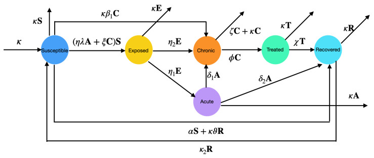
Hepatitis B is a worldwide viral infection that causes cirrhosis, hepatocellular cancer, the need for liver transplantation, and death. This work proposed a mathematical representation of Hepatitis B Virus (HBV) transmission traits emphasizing the significance of applied mathematics in comprehending how the disease spreads. The work used an updated Atangana-Baleanu fractional difference operator to create a fractional-order model of HBV. The qualitative assessment and well-posedness of the mathematical framework were looked at, and the global stability of equilibrium states as measured by the Volterra-type Lyapunov function was summarized. The exact answer was guaranteed to be unique using the Lipschitz condition. Additionally, there were various analyses of this new type of operator to support the operator's efficacy. We observe that the explored discrete fractional operators will be $ \chi^2 $-increasing or decreasing in certain domains of the time scale $ \mathbb{N}_j: = {j, j + 1, ... } $ by looking at the fundamental characteristics of the proposed discrete fractional operators along with $ \chi $-monotonicity descriptions. For numerical simulations, solutions were constructed in the discrete generalized form of the Mittag-Leffler kernel, highlighting the impacts of the illness caused by numerous causes. The order of the fractional derivative had a significant influence on the dynamical process utilized to construct the HBV model. Researchers and policymakers can benefit from the suggested model's ability to forecast infectious diseases such as HBV and take preventive action.
- Hepatitis B model,
- discrete Mittag-Leffler kernel,
- $ \chi $-monotonicity investigations,
- Volterra-type Lyapunov function
Citation: Muhammad Farman, Ali Akgül, J. Alberto Conejero, Aamir Shehzad, Kottakkaran Sooppy Nisar, Dumitru Baleanu. Analytical study of a Hepatitis B epidemic model using a discrete generalized nonsingular kernel[J]. AIMS Mathematics, 2024, 9(7): 16966-16997. doi: 10.3934/math.2024824

Related Papers:

Abstract

Hepatitis B is a worldwide viral infection that causes cirrhosis, hepatocellular cancer, the need for liver transplantation, and death. This work proposed a mathematical representation of Hepatitis B Virus (HBV) transmission traits emphasizing the significance of applied mathematics in comprehending how the disease spreads. The work used an updated Atangana-Baleanu fractional difference operator to create a fractional-order model of HBV. The qualitative assessment and well-posedness of the mathematical framework were looked at, and the global stability of equilibrium states as measured by the Volterra-type Lyapunov function was summarized. The exact answer was guaranteed to be unique using the Lipschitz condition. Additionally, there were various analyses of this new type of operator to support the operator's efficacy. We observe that the explored discrete fractional operators will be $ \chi^2 $-increasing or decreasing in certain domains of the time scale $ \mathbb{N}_j: = {j, j + 1, ... } $ by looking at the fundamental characteristics of the proposed discrete fractional operators along with $ \chi $-monotonicity descriptions. For numerical simulations, solutions were constructed in the discrete generalized form of the Mittag-Leffler kernel, highlighting the impacts of the illness caused by numerous causes. The order of the fractional derivative had a significant influence on the dynamical process utilized to construct the HBV model. Researchers and policymakers can benefit from the suggested model's ability to forecast infectious diseases such as HBV and take preventive action.

References

[1]	F. A. Wodajo, T. T. Mekonnen, Effect of intervention of vaccination and treatment on the transmission dynamics of HBV disease: A mathematical model analysis, J. Math., 2022, 1–17. https://doi.org/10.1155/2022/9968832
[2]	S. Tsukuda, K. Watashi, Hepatitis B virus biology and life cycle, Antiviral Res., 182 (2020), 104925. https://doi.org/10.1016/j.antiviral.2020.104925 doi: 10.1016/j.antiviral.2020.104925
[3]	E. E. Conners, L. Panagiotakopoulos, M. G. Hofmeister, P. R. Spradling, L. M. Hagan, A. M. Harris, et al., Screening and testing for hepatitis B virus infection: CDC recommendations-United States, 2023, MMWR Recomm. Rep., 72 (2023), 1.
[4]	J. E. Flores, A. J. Thompson, M. Ryan, J. Howell, The global impact of hepatitis B vaccination on hepatocellular carcinoma, Vaccines, 10 (2022), 793. https://doi.org/10.3390/vaccines10050793 doi: 10.3390/vaccines10050793
[5]	N. Chitnis, J. M. Hyman, J. M. Cushing, Determining important parameters in the spread of malaria through the sensitivity analysis of a mathematical model, Bull. Math. Bol., 70 (2008), 1272–1296. https://doi.org/10.1007/s11538-008-9299-0 doi: 10.1007/s11538-008-9299-0
[6]	J. P. Chretien, S. Riley, D. B. George, Mathematical modeling of the West Africa Ebola epidemic, Elife, 4 (2015), e09186. https://doi.org/10.7554/eLife.09186 doi: 10.7554/eLife.09186
[7]	M. F. Tabassum, M. Saeed, A. Akgül, M. Farman, N. A. Chaudhry, Treatment of HIV/AIDS epidemic model with vertical transmission by using evolutionary Padé-approximation, Chaos Soliton. Fract., 134 (2020), 109686.
[8]	M. Farman, A. Shehzad, A. Akgül, D. Baleanu, M. D. L. Sen, Modelling and analysis of a measles epidemic model with the constant proportional Caputo operator, Symmetry, 15 (2023), 468. https://doi.org/10.3390/sym15020468 doi: 10.3390/sym15020468
[9]	S. Zhao, Z. Xu, Y. Lu, A mathematical model of hepatitis B virus transmission and its application for vaccination strategy in China, Int. J. Epidemiol., 29 (2000), 744–752.
[10]	K. Wang, W. Wang, Propagation of HBV with spatial dependence, Math. Biosci., 210 (2007), 78–95. https://doi.org/10.1016/j.mbs.2007.05.004 doi: 10.1016/j.mbs.2007.05.004
[11]	N. K. Martin, P. Vickerman, M. Hickman, Mathematical modelling of hepatitis C treatment for injecting drug users, J. Theor. Biol., 274 (2011), 58–66. https://doi.org/10.1016/j.jtbi.2010.12.041 doi: 10.1016/j.jtbi.2010.12.041
[12]	A. V. Kamyad, R. Akbari, A. A. Heydari, A. Heydari, Mathematical modeling of transmission dynamics and optimal control of vaccination and treatment for hepatitis B virus, Comput. Math. Methods Med., 2014 (2014), 475451. https://doi.org/10.1155/2014/475451 doi: 10.1155/2014/475451
[13]	S. Ullah, M. A. Khan, J. F. Gómez-Aguilar, Mathematical formulation of hepatitis B virus with optimal control analysis, Optim. Control Appl. Methods, 40 (2019), 529–544. https://doi.org/10.1002/oca.2493 doi: 10.1002/oca.2493
[14]	F. A. Wodajo, D. M. Gebru, H. T. Alemneh, Mathematical model analysis of effective intervention strategies on transmission dynamics of hepatitis B virus, Sci. Rep., 13 (2023), 8737. https://doi.org/10.1038/s41598-023-35815-z doi: 10.1038/s41598-023-35815-z
[15]	M. Farman, C. Alfiniyah, A. Shehzad, Modelling and analysis tuberculosis (TB) model with hybrid fractional operator, Alex. Eng. J., 72 (2023), 463–478. https://doi.org/10.1016/j.aej.2023.04.017 doi: 10.1016/j.aej.2023.04.017
[16]	F. E. Guma, O. M. Badawy, M. Berir, M. A. Abdoon, Numerical analysis of fractional-order dynamic dengue disease epidemic in Sudan, J. Niger. Soc. Phys. Sci., 5 (2023), 1464–1464. https://doi.org/10.46481/jnsps.2023.1464 doi: 10.46481/jnsps.2023.1464
[17]	C. Xu, M. Farman, A. Hasan, A. Akgül, M. Zakarya, W. Albalawi, et al., Lyapunov stability and wave analysis of COVID-19 omicron variant of real data with fractional operator, Alex. Eng. J., 61 (2022), 11787–11802. https://doi.org/10.1016/j.aej.2022.05.025 doi: 10.1016/j.aej.2022.05.025
[18]	Y. Gu, M. Khan, R. Zarin, A. Khan, A. Yusuf, U. W. Humphries, Mathematical analysis of a new nonlinear dengue epidemic model via deterministic and fractional approach, Alex. Eng. J., 67 (2023), 1–21. https://doi.org/10.1016/j.aej.2022.10.057 doi: 10.1016/j.aej.2022.10.057
[19]	M. Farman, S. Jamil, K. S. Nisar, A. Akgül, Mathematical study of fractal-fractional leptospirosis disease in human and rodent populations dynamical transmission, Ain Shams Eng. J., 15 (2024), 102452. https://doi.org/10.1016/j.asej.2023.102452 doi: 10.1016/j.asej.2023.102452
[20]	K. Wang, C. Wei, Fractal soliton solutions for the fractal-fractional shallow water wave equation arising in ocean engineering, Alex. Eng. J., 65 (2023), 859–865. https://doi.org/10.1016/j.aej.2022.10.024 doi: 10.1016/j.aej.2022.10.024
[21]	K. A. Abro, A. Atangana, J. F. Gomez-Aguilar, Optimal synchronization of fractal-fractional differentials on chaotic convection for Newtonian and non-Newtonian fluids, Eur. Phys. J. Spec. Top., 232 (2023), 2403–2414. https://doi.org/10.1140/epjs/s11734-023-00913-6 doi: 10.1140/epjs/s11734-023-00913-6
[22]	I. Dassios, T. Kërçi, D. Baleanu, F. Milano, Fractional-order dynamical model for electricity markets, Math. Method. Appl. Sci., 46 (2023), 8349–8361. https://doi.org/10.1002/mma.7892 doi: 10.1002/mma.7892
[23]	J. A. Conejero, J. Franceschi, E. Picó-Marco, Fractional vs. ordinary control systems: What does the fractional derivative provide? Mathematics, 10 (2022), 2719.
[24]	C. Xu, D. Mu, Z. Liu, Y. Pang, C. Aouiti, O. Tunc, et al., Bifurcation dynamics and control mechanism of a fractional-order delayed Brusselator chemical reaction model, Match, 89 (2023). https://doi.org/10.46793/match.89-1.073X
[25]	L. C. Cardoso, F. L. P. Dos Santos, R. F. Camargo, Analysis of fractional-order models for hepatitis B, Comput. Appl. Math., 37 (2018), 4570–4586. https://doi.org/10.1007/s40314-018-0588-4 doi: 10.1007/s40314-018-0588-4
[26]	M. A. Khan, Z. Hammouch, D. Baleanu, Modeling the dynamics of hepatitis E via the Caputo-Fabrizio derivative, Math. Model Nat. Phenom., 14 (2019), 311. https://doi.org/10.1051/mmnp/2018074 doi: 10.1051/mmnp/2018074
[27]	S. A. A. Shah, M. A. Khan, M. Farooq, S. Ullah, E. O. Alzahrani, A fractional order model for Hepatitis B virus with treatment via Atangana-Baleanu derivative, Physica A, 538 (2020), 122636. https://doi.org/10.1016/j.physa.2019.122636 doi: 10.1016/j.physa.2019.122636
[28]	F. Gao, X. Li, W. Li, X. Zhou, Stability analysis of a fractional-order novel hepatitis B virus model with immune delay based on Caputo-Fabrizio derivative, Chaos Soliton. Fract., 142 (2021), 110436. https://doi.org/10.1016/j.chaos.2020.110436 doi: 10.1016/j.chaos.2020.110436
[29]	X. P. Li, A. Din, A. Zeb, S. Kumar, T. Saeed, The impact of Lévy noise on a stochastic and fractal-fractional Atangana-Baleanu order hepatitis B model under real statistical data, Chaos Soliton. Fract., 154 (2022), 111623.
[30]	J. Lin, J. Bai, S. Reutskiy, J. Lu, A novel RBF-based meshless method for solving time-fractional transport equations in 2D and 3D arbitrary domains, Eng. Comput., 39 (2023), 1905–1922. https://doi.org/10.1007/s00366-022-01601-0 doi: 10.1007/s00366-022-01601-0
[31]	T. Abdeljawad, D. Baleanu, Discrete fractional differences with nonsingular discrete Mittag-Leffler kernels, Adv. Differ. Eq., 2016 (2016), 1–18. https://doi.org/10.1186/s13662-016-0949-5 doi: 10.1186/s13662-016-0949-5
[32]	T. Abdeljawad, Fractional difference operators with discrete generalized Mittag-Leffler kernels, Chaos Soliton. Fract., 126 (2019), 315–324. https://doi.org/10.1016/j.chaos.2019.06.012 doi: 10.1016/j.chaos.2019.06.012
[33]	P. O. Mohammed, H. M. Srivastava, D. Baleanu, K. M. Abualnaja, Modified fractional difference operators defined using Mittag-Leffler kernels, Symmetry, 14 (2022), 1519. https://doi.org/10.3390/sym14081519 doi: 10.3390/sym14081519
[34]	M. Farman, A. Shehzad, A. Akgül, D. Baleanu, N. Attia, A. M. Hassan, Analysis of a fractional order Bovine Brucellosis disease model with discrete generalized Mittag-Leffler kernels, Res. Phys., 52 (2023), 106887. https://doi.org/10.1016/j.rinp.2023.106887 doi: 10.1016/j.rinp.2023.106887
[35]	G. Narayanan, M. S. Ali, G. Rajchakit, A. Jirawattanapanit, B. Priya, Stability analysis for Nabla discrete fractional-order of Glucose-Insulin Regulatory System on diabetes mellitus with Mittag-Leffler kernel, Biomed. Signal Proces., 80 (2023), 104295. https://doi.org/10.1016/j.bspc.2022.104295 doi: 10.1016/j.bspc.2022.104295
[36]	T. Abdeljawad, On delta and nabla Caputo fractional differences and dual identities, Discrete Dyn. Nat. Soc., 2013 (2013). https://doi.org/10.1155/2013/406910
[37]	T. Abdeljawad, F. Jarad, D. Baleanu, A semigroup-like property for discrete Mittag-Leffler functions, Adv. Diff. Eq., 2012 (2012), 1–7.
[38]	T. Abdeljawad, D. Baleanu, Monotonicity analysis of a nabla discrete fractional operator with discrete Mittag-Leffler kernel, Chaos Soliton. Fract., 102 (2017), 106–110. https://doi.org/10.1186/1687-1847-2012-72 doi: 10.1186/1687-1847-2012-72
[39]	P. O. Mohammed, H. M. Srivastava, D. Baleanu, K. M. Abualnaja, Modified fractional difference operators defined using Mittag-Leffler kernels, Symmetry, 14 (2022), 1519. https://doi.org/10.3390/sym14081519
[40]	P. O. Mohammed, C. S. Goodrich, A. B. Brzo, Y. S. Hamed, New classifications of monotonicity investigation for discrete operators with Mittag-Leffler kernel, Math. Biosci. Eng., 19 (2022), 4062–4074. https://doi.org/10.3934/mbe.2022186 doi: 10.3934/mbe.2022186
[41]	C. Vargas-De-León, Volterra-type Lyapunov functions for fractional-order epidemic systems, Commun. Nonlinear Sci. Numer. Simul., 24 (2015), 75–85. https://doi.org/10.1016/j.cnsns.2014.12.013 doi: 10.1016/j.cnsns.2014.12.013

Reader Comments

Your name:*

Email:*
© 2024 the Author(s), licensee AIMS Press. This is an open access article distributed under the terms of the Creative Commons Attribution License (http://creativecommons.org/licenses/by/4.0)