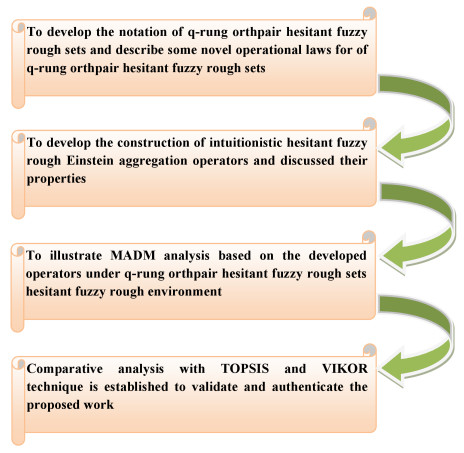
Environmental science and pollution research has benefits around the globe. Human activity produces more garbage throughout the day as the world's population and lifestyles rise. Choosing a garbage disposal site (GDS) is crucial to effective disposal. In illuminated of the advancements in society, decision-makers concede a significant challenge for assessing an appropriate location for a garbage disposal site. This research used a multi-attribute decision-making (MADM) approach based on $ q $-rung orthopair hesitant fuzzy rough ($ q $-ROHFR) Einstein aggregation information for evaluating GDS selection schemes and providing decision-making (DM) support to select a suitable waste disposal site. In this study, first, q-ROHFR Einstein average aggregation operators are integrated. Some intriguing characteristics of the suggested operators, such as monotonicity, idempotence and boundedness were also explored. Then, a MADM technique was established using the novel concept of $ q $-ROHFR aggregation operators under Einstein t-norm and t-conorm. In order to help the decision makers (DMs) make a final choice, this technique aims to rank and choose an alternative from a collection of feasible alternatives, as well as to propose a solution based on the ranking of alternatives for a problem with conflicting criteria. The model's adaptability and validity are then demonstrated by an analysis and solution of a numerical issue involving garbage disposal plant site selection. We performed a the sensitivity analysis of the proposed aggregation operators to determine the outcomes of the decision-making procedure. To highlight the potential of our new method, we performed a comparison study using the novel extended TOPSIS and VIKOR schemes based on $ q $-ROHFR information. Furthermore, we compared the results with those existing in the literature. The findings demonstrate that this methodology has a larger range of information representation, more flexibility in the assessment environment, and improved consistency in evaluation results.
Citation: Attaullah, Asghar Khan, Noor Rehman, Fuad S. Al-Duais, Afrah Al-Bossly, Laila A. Al-Essa, Elsayed M Tag-eldin. A novel decision model with Einstein aggregation approach for garbage disposal plant site selection under $ q $-rung orthopair hesitant fuzzy rough information[J]. AIMS Mathematics, 2023, 8(10): 22830-22874. doi: 10.3934/math.20231163
Environmental science and pollution research has benefits around the globe. Human activity produces more garbage throughout the day as the world's population and lifestyles rise. Choosing a garbage disposal site (GDS) is crucial to effective disposal. In illuminated of the advancements in society, decision-makers concede a significant challenge for assessing an appropriate location for a garbage disposal site. This research used a multi-attribute decision-making (MADM) approach based on $ q $-rung orthopair hesitant fuzzy rough ($ q $-ROHFR) Einstein aggregation information for evaluating GDS selection schemes and providing decision-making (DM) support to select a suitable waste disposal site. In this study, first, q-ROHFR Einstein average aggregation operators are integrated. Some intriguing characteristics of the suggested operators, such as monotonicity, idempotence and boundedness were also explored. Then, a MADM technique was established using the novel concept of $ q $-ROHFR aggregation operators under Einstein t-norm and t-conorm. In order to help the decision makers (DMs) make a final choice, this technique aims to rank and choose an alternative from a collection of feasible alternatives, as well as to propose a solution based on the ranking of alternatives for a problem with conflicting criteria. The model's adaptability and validity are then demonstrated by an analysis and solution of a numerical issue involving garbage disposal plant site selection. We performed a the sensitivity analysis of the proposed aggregation operators to determine the outcomes of the decision-making procedure. To highlight the potential of our new method, we performed a comparison study using the novel extended TOPSIS and VIKOR schemes based on $ q $-ROHFR information. Furthermore, we compared the results with those existing in the literature. The findings demonstrate that this methodology has a larger range of information representation, more flexibility in the assessment environment, and improved consistency in evaluation results.

| [1] |
Z. Raizah, U. K. K. Nanjappa, H. U. A. Shankar, U. Khan, S. M. Eldin, R. Kumar, et al., Windmill global sourcing in an initiative using a spherical fuzzy multiple-criteria decision prototype, Energies, 15 (2022), 8000. https://doi.org/10.3390/en15218000 doi: 10.3390/en15218000

|
| [2] |
M. M. Lashin, M. I. Khan, N. B. Khedher, S. M. Eldin, Optimization of display window design for females clothes for fashion stores through artificial intelligence and fuzzy system, Appl. Sci., 12 (2022), 11594. https://doi.org/10.3390/app122211594 doi: 10.3390/app122211594
|
| [3] |
G. Shahzadi, F. Zafar, M. A. Alghamdi, Multiple-attribute decision-making using Fermatean fuzzy Hamacher interactive geometric operators, Math. Prob. Eng., 2021, 1–20. https://doi.org/10.1155/2021/5150933 doi: 10.1155/2021/5150933
|
| [4] |
S. Ashraf, S. N. Abbasi, M. Naeem, S. M. Eldin, Novel decision aid model for green supplier selection based on extended EDAS approach under pythagorean fuzzy Z-numbers, Front. Env. Sci., 11 (2023), 342. https://doi.org/10.3389/fenvs.2023.1137689 doi: 10.3389/fenvs.2023.1137689
|
| [5] |
Attaullah, S. Ashraf, N. Rehman, A. Khan, M. Naeem, C. Park, A wind power plant site selection algorithm based on q-rung orthopair hesitant fuzzy rough Einstein aggregation information, Sci. Rep., 12 (2022), 5443. https://doi.org/10.1038/s41598-022-09323-5 doi: 10.1038/s41598-022-09323-5
|
| [6] |
Attaullah, S. Ashraf, N. Rehman, H. AlSalman, A. H. Gumaei, A decision-making framework using q-rung orthopair probabilistic hesitant fuzzy rough aggregation information for the drug selection to treat COVID-19, Complexity, 2022. https://doi.org/10.1155/2022/5556309 doi: 10.1155/2022/5556309
|
| [7] |
Attaullah, S. Ashraf, N. Rehman, A. Khan, C. Park, A decision making algorithm for wind power plant based on q-rung orthopair hesitant fuzzy rough aggregation information and TOPSIS, AIMS Math., 7 (2022), 5241–5274. https://doi.org/10.3934/math.2022292 doi: 10.3934/math.2022292
|
| [8] |
Attaullah, N. Rehman, A. Khan, G. Santos-Garcia, Fermatean hesitant fuzzy rough aggregation operators and their applications in multiple criteria group decision-making, Sci. Rep., 13 (2023), 6676. https://doi.org/10.1038/s41598-023-28722-w doi: 10.1038/s41598-023-28722-w
|
| [9] |
V. Nevrlý, R. Šomplák, O. Putna, M. Pavlas, Location of mixed municipal waste treatment facilities: Cost of reducing greenhouse gas emissions, J. Clean. Prod., 239 (2019), 118003. https://doi.org/10.1016/j.jclepro.2019.118003 doi: 10.1016/j.jclepro.2019.118003
|
| [10] |
A. Kumar, S. R. Samadder, A review on technological options of waste to energy for effective management of municipal solid waste, Waste Manage., 69 (2017), 407–422. https://doi.org/10.1016/j.wasman.2017.08.046 doi: 10.1016/j.wasman.2017.08.046
|
| [11] |
J. Song, Y. Sun, L. Jin, PESTEL analysis of the development of the waste-to-energy incineration industry in China, Renew. Sust. Energ. Rev., 80 (2017), 276–289. https://doi.org/10.1016/j.rser.2017.05.066 doi: 10.1016/j.rser.2017.05.066
|
| [12] |
H. Jiang, J. Zhan, D. Chen, PROMETHEE-Ⅱ method based on variable precision fuzzy rough sets with fuzzy neighborhoods, Artif. Intell. Rev., 54 (2021), 1281–1319. https://doi.org/10.1007/s10462-020-09878-7 doi: 10.1007/s10462-020-09878-7
|
| [13] |
L. A. Zadeh, Fuzzy sets, Inform. Control, 8 (1965), 338–353. https://doi.org/10.1016/S0019-9958(65)90241-X doi: 10.1016/S0019-9958(65)90241-X
|
| [14] | K. T. Atanassov, Intuitionistic fuzzy sets, In: Intuitionistic fuzzy sets, 1999, 1–137, Physica, Heidelberg. https://doi.org/10.1007/978-3-7908-1870-3_1 |
| [15] |
S. Singh, S. Sharma, S. Lalotra, Generalized correlation coefficients of intuitionistic fuzzy sets with application to MAGDM and clustering analysis, Int. J. Fuzzy Syst., 22 (2020), 1582–1595. https://doi.org/10.3390/e23050563 doi: 10.3390/e23050563
|
| [16] |
R. R. Yager, A. M. Abbasov, Pythagorean membership grades, complex numbers, and decision making, Int. J. Intell. Syst., 28 (2013), 436–452. https://doi.org/10.1002/int.21584 doi: 10.1002/int.21584
|
| [17] |
O. Yanmaz, Y. Turgut, E. N. Can, C. Kahraman, Interval-valued Pythagorean fuzzy EDAS method: An application to car selection problem, J. Intell. Fuzzy Syst., 38 (2020), 4061–4077. https://doi.org/10.3233/JIFS-182667 doi: 10.3233/JIFS-182667
|
| [18] |
R. R. Yager, Generalized orthopair fuzzy sets, IEEE T. Fuzzy Syst., 25 (2016), 1222–1230. https://doi.org/10.1109/TFUZZ.2016.2604005 doi: 10.1109/TFUZZ.2016.2604005
|
| [19] |
C. Zhang, J. Ding, D. Li, J. Zhan, A novel multi-granularity three-way decision making approach in q-rung orthopair fuzzy information systems, Int. J. Approx. Reason., 138 (2021), 161–187. https://doi.org/10.1016/j.ijar.2021.08.004 doi: 10.1016/j.ijar.2021.08.004
|
| [20] |
C. Zhang, J. Ding, J. Zhan, A. K. Sangaiah, D. Li, Fuzzy intelligence learning based on bounded rationality in IoMT systems: A case study in Parkinson Disease, IEEE T. Comput. Soc. Syst., 2022. https://doi.org/10.1109/TCSS.2022.3221933 doi: 10.1109/TCSS.2022.3221933
|
| [21] |
C. Zhang, W. Bai, D. Li, J. Zhan, Multiple attribute group decision making based on multigranulation probabilistic models, MULTIMOORA and TPOP in incomplete q-rung orthopair fuzzy information systems, Int. J. Approx. Reason., 143 (2022), 102–120. https://doi.org/10.1016/j.ijar.2022.01.002 doi: 10.1016/j.ijar.2022.01.002
|
| [22] |
A. Hussain, M. I. Ali, T. Mahmood, Covering based q-rung orthopair fuzzy rough set model hybrid with TOPSIS for multi-attribute decision making, J. Intell. Fuzzy Syst., 37 (2019), 981–993. https://doi.org/10.3233/JIFS-181832 doi: 10.3233/JIFS-181832
|
| [23] |
S. Chakraborty, TOPSIS and modified TOPSIS: A comparative analysis, Decis. Anal. J., 2 (2022), 100021. https://doi.org/10.1016/j.dajour.2021.100021 doi: 10.1016/j.dajour.2021.100021
|
| [24] |
M. Hanine, O. Boutkhoum, A. Tikniouine, T. Agouti, Application of an integrated multi-criteria decision making AHP-TOPSIS methodology for ETL software selection, SpringerPlus, 5 (2016), 1–17. https://doi.org/10.1186/s40064-016-2233-2 doi: 10.1186/s40064-016-2233-2
|
| [25] |
P. Gupta, M. K. Mehlawat, N. Grover, Intuitionistic fuzzy multi-attribute group decision-making with an application to plant location selection based on a new extended VIKOR method, Inform. Sci., 370 (2016), 184–203. https://doi.org/10.1016/j.ins.2016.07.058 doi: 10.1016/j.ins.2016.07.058
|
| [26] |
A. Hafezalkotob, A. Hafezalkotob, Interval target-based VIKOR method supported on interval distance and preference degree for machine selection, Eng. Appl. Artif. Intel., 57 (2017), 184–196. https://doi.org/10.1016/j.engappai.2016.10.018 doi: 10.1016/j.engappai.2016.10.018
|
| [27] |
O. Soner, E. Celik, E. Akyuz, Application of AHP and VIKOR methods under interval type 2 fuzzy environment in maritime transportation, Ocean Eng., 129 (2017), 107–116. https://doi.org/10.3390/math11102249 doi: 10.3390/math11102249
|
| [28] |
M. Gul, E. Celik, N. Aydin, A. T. Gumus, A. F. Guneri, A state of the art literature review of VIKOR and its fuzzy extensions on applications, Appl. Soft Comput., 46 (2016), 60–89. https://doi.org/10.1016/j.asoc.2016.04.040 doi: 10.1016/j.asoc.2016.04.040
|
| [29] |
S. Opricovic, G. H. Tzeng, Extended VIKOR method in comparison with outranking methods, Eur. J. Oper. Res., 178 (2007), 514–529. https://doi.org/10.1016/j.ejor.2006.01.020 doi: 10.1016/j.ejor.2006.01.020
|
| [30] |
Z. Pawlak, Rough sets, Int. J. Comput. Inform. Sci., 11 (1982), 341–356. https://doi.org/10.1007/BF01001956 doi: 10.1016/j.ins.2021.04.016
|
| [31] |
T. M. Al-shami, An improvement of rough sets accuracy measure using containment neighborhoods with a medical application, Inform. Sci., 569 (2021), 110–124. https://doi.org/10.1016/j.ins.2021.04.016 doi: 10.1016/j.ins.2021.04.016
|
| [32] |
Z. Pawlak, A. Skowron, Rudiments of rough sets, Inform. Sci., 177 (2007), 3–27. https://doi.org/10.1016/j.ins.2006.06.003 doi: 10.1016/j.ins.2006.06.003
|
| [33] |
S. Sadek, M. El-Fadel, F. Freiha, Compliance factors within a GIS-based framework for landfill siting, Int. J. Env. Stud., 63 (2006), 71–86. https://doi.org/10.1080/00207230600562213 doi: 10.1080/00207230600562213
|
| [34] |
A. M. Radzikowska, E. E. Kerre, A comparative study of fuzzy rough sets, Fuzzy Set. Syst., 126 (2002), 137–155. https://doi.org/10.1016/S0165-0114(01)00032-X doi: 10.1016/S0165-0114(01)00032-X
|
| [35] |
W. Pan, K. She, P. Wei, Multi-granulation fuzzy preference relation rough set for ordinal decision system, Fuzzy Set. Syst., 312 (2017), 87–108. https://doi.org/10.1016/j.fss.2016.08.002 doi: 10.1016/j.fss.2016.08.002
|
| [36] |
Y. Li, S. Wu, Y. Lin, J. Liu, Different classes' ratio fuzzy rough set based robust feature selection, Knowl.-Based Syst., 120 (2017), 74–86. https://doi.org/10.1155/2021/6685396 doi: 10.1155/2021/6685396
|
| [37] |
T. Zhan, Granular-based state estimation for nonlinear fractional control systems and its circuit cognitive application, Int. J. Cogn. Comput. Eng., 4 (2023), 1–5. https://doi.org/10.1016/j.ijcce.2022.12.001 doi: 10.1016/j.ijcce.2022.12.001
|
| [38] |
X. Ren, D. Li, Y. Zhai, Research on mixed decision implications based on formal concept analysis, Int. J. Cogn. Comput. Eng., 4 (2023), 71–77. https://doi.org/10.1016/j.ijcce.2023.02.007 doi: 10.1016/j.ijcce.2023.02.007
|
| [39] |
K. Lian, T. Wang, B. Wang, M. Wang, W. Huang, J. Yang, The research on relative knowledge distances and their cognitive features, Int. J. Cogn. Comput. Eng., 2023. https://doi.org/10.1016/j.ijcce.2023.03.004 doi: 10.1016/j.ijcce.2023.03.004
|
| [40] |
T. Feng, H. T. Fan, J. S. Mi, Uncertainty and reduction of variable precision multigranulation fuzzy rough sets based on three-way decisions, Int. J. Approx. Reason., 85 (2017), 36–58. https://doi.org/10.1016/j.ins.2022.05.122 doi: 10.1016/j.ins.2022.05.122
|
| [41] |
B. Sun, W. Ma, X. Chen, X. Zhang, Multigranulation vague rough set over two universes and its application to group decision making, Soft Comput., 23 (2019), 8927–8956. https://doi.org/10.1007/s00500-018-3494-1 doi: 10.1007/s00500-018-3494-1
|
| [42] |
C. Y. Wang, B. Q. Hu, Granular variable precision fuzzy rough sets with general fuzzy relations, Fuzzy Set. Syst., 275 (2015), 39–57. https://doi.org/10.1007/s40314-023-02245-6 doi: 10.1007/s40314-023-02245-6
|
| [43] |
S. Vluymans, D. S. Tarragó, Y. Saeys, C. Cornelis, F. Herrera, Fuzzy rough classifiers for class imbalanced multi-instance data, Pattern Recog., 53 (2016), 36–45. https://doi.org/10.1016/j.patcog.2015.12.002 doi: 10.1016/j.patcog.2015.12.002
|
| [44] |
C. Y. Wang, B. Q. Hu, Fuzzy rough sets based on generalized residuated lattices, Inform. Sci., 248 (2013), 31–49. https://doi.org/10.1016/j.ins.2013.03.051 doi: 10.1016/j.ins.2013.03.051
|
| [45] |
H. Zhang, L. Shu, S. Liao, C. Xiawu, Dual hesitant fuzzy rough set and its application, Soft Comput., 21 (2017), 3287–3305. https://doi.org/10.1007/s00500-015-2008-7 doi: 10.1007/s00500-015-2008-7
|
| [46] |
D. Peng, J. Wang, D. Liu, Y. Cheng, The interactive fuzzy linguistic term set and its application in multi-attribute decision making, Artif. Intell. Medicine, 131 (2022), 102345. https://doi.org/10.1016/j.artmed.2022.102345 doi: 10.1016/j.artmed.2022.102345
|
| [47] |
D. Peng, J. Wang, D. Liu, Z. Liu, An improved EDAS method for the multi-attribute decision making based on the dynamic expectation level of decision makers, Symmetry, 14 (2022), 979. https://doi.org/10.3390/sym14050979 doi: 10.3390/sym14050979
|
| [48] |
G. Tang, F. Chiclana, P. Liu, A decision-theoretic rough set model with q-rung orthopair fuzzy information and its application in stock investment evaluation, Appl. Soft Comput., 91 (2020), 106212. https://doi.org/10.1016/j.asoc.2020.106212 doi: 10.1016/j.asoc.2020.106212
|
| [49] |
D. Liang, W. Cao, q-Rung orthopair fuzzy sets-based decision-theoretic rough sets for three-way decisions under group decision making, Int. J. Intell. Syst., 34 (2019), 3139–3167. https://doi.org/10.1002/int.22187 doi: 10.1002/int.22187
|
| [50] | Z. Zhang, S. M. Chen, Group decision making with incomplete q-rung orthopair fuzzy preference relations, Inform. Sci., 553 (2021), 376–396. |
| [51] |
D. Peng, J. Wang, D. Liu, Z. Liu, The similarity measures for linguistic q-rung orthopair fuzzy multi-criteria group decision making using projection method, IEEE Access, 7 (2019), 176732–176745. https://doi.org/10.1109/ACCESS.2019.2957916 doi: 10.1109/ACCESS.2019.2957916
|
| [52] |
K. Charnpratheep, Q. Zhou, B. Garner, Preliminary landfill site screening using fuzzy geographical information systems, Waste Manag. Res., 15 (1997), 197–215. https://doi.org/10.1177/0734242X9701500207 doi: 10.1177/0734242X9701500207
|
| [53] |
O. E. Demesouka, A. P Vavatsikos, K. P. Anagnostopoulos, Suitability analysis for siting MSW landfills and its multicriteria spatial decision support system: Method, implementation and case study, Waste Manage., 33 (2013), 1190–1206. https://doi.org/10.1016/j.wasman.2013.01.030 doi: 10.1016/j.wasman.2013.01.030
|
| [54] |
M. Ekmekçioǧlu, T. Kaya, C. Kahraman, Fuzzy multicriteria disposal method and site selection for municipal solid waste, Waste Manage., 30 (2010), 1729–1736. https://doi.org/10.1016/j.wasman.2010.02.031 doi: 10.1016/j.wasman.2010.02.031
|
| [55] |
S. Ashraf, N. Rehman, A. Hussain, H. AlSalman, A. H. Gumaei, q-Rung orthopair fuzzy 380 rough Einstein aggregation information-based EDAS method: Applications in robotic agrifarming, Comput. Intell. Neurosci., 2021. https://doi.org/10.1155/2021/5520264 doi: 10.1155/2021/5520264
|
| [56] |
P. F. Hsu, M. G. Hsu, Optimizing the information outsourcing practices of primary care medical organizations using entropy and TOPSIS, Qual. Quant., 42 (2008), 181–201. https://doi.org/10.1007/s11135-006-9040-8 doi: 10.1007/s11135-006-9040-8
|
| [57] | C. L. Hwang, K. Yoon, Methods for multiple attribute decision making, In: Multiple attribute decision making, 1981, 58–191. Springer, Berlin, Heidelberg. https://doi.org/10.1007/978-3-642-48318-9_3 |
| [58] |
D. Liu, D. Peng, Z. Liu, The distance measures between q-rung orthopair hesitant fuzzy sets and their application in multiple criteria decision making, Int. J. Intell. Syst., 34 (2019), 2104–2121. https://doi.org/10.1002/int.22133 doi: 10.1002/int.22133
|
| [59] | G. H. Tzeng, J. J. Huang, Multiple attribute decision making: Methods and applications, CRC Press, 2011. https://doi.org/10.1201/b11032 |


Figures(6) / Tables(27)

Attaullah, Asghar Khan, Noor Rehman, Fuad S. Al-Duais, Afrah Al-Bossly, Laila A. Al-Essa, Elsayed M Tag-eldin. A novel decision model with Einstein aggregation approach for garbage disposal plant site selection under $ q $-rung orthopair hesitant fuzzy rough information[J]. AIMS Mathematics, 2023, 8(10): 22830-22874. doi: 10.3934/math.20231163


 DownLoad: