A linearly convergent proximal ADMM with new iterative format for BPDN in compressed sensing problem

Bing Xue; Jiakang Du; Hongchun Sun; Yiju Wang; Bing Xue; Jiakang Du; Hongchun Sun; Yiju Wang

doi:10.3934/math.2022586

AIMS Mathematics

2022, Volume 7, Issue 6: 10513-10533. doi: 10.3934/math.2022586

Previous Article Next Article

Research article

A linearly convergent proximal ADMM with new iterative format for BPDN in compressed sensing problem

Bing Xue ¹,
Jiakang Du ²,
Hongchun Sun ^{1
,
,},
Yiju Wang ^{2
,
,}

1.
School of Mathematics and Statistics, Linyi University, Linyi 276005, China
2.
School of Management Science, Qufu Normal University, Rizhao 276800, China

Received: 18 December 2021 Revised: 11 March 2022 Accepted: 15 March 2022 Published: 28 March 2022
MSC : 90C30, 90C33

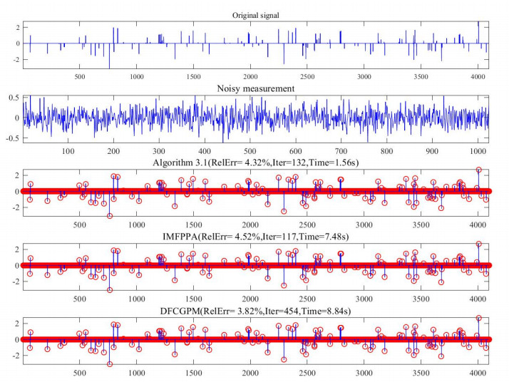
In recent years, compressive sensing (CS) problem is being popularly applied in the fields of signal processing and statistical inference. The alternating direction method of multipliers (ADMM) is applicable to the equivalent forms of basis pursuit denoising (BPDN) in CS problem. However, the solving speed and accuracy are adversely affected when the dimension increases greatly. In this paper, a new iterative format of proximal ADMM, which has fast solving speed and pinpoint accuracy when the dimension increases, is proposed to solve BPDN problem. Global convergence of the new type proximal ADMM is established in detail, and we exhibit a $ R- $ linear convergence rate under suitable condition. Moreover, we apply this new algorithm to solve different types of BPDN problems. Compared with the state-of-the-art of algorithms in BPDN problem, the proposed algorithm is more accurate and efficient.
- new type proximal ADMM,
- global convergence,
- $ R- $ linear convergence rate,
- BPDN problem
Citation: Bing Xue, Jiakang Du, Hongchun Sun, Yiju Wang. A linearly convergent proximal ADMM with new iterative format for BPDN in compressed sensing problem[J]. AIMS Mathematics, 2022, 7(6): 10513-10533. doi: 10.3934/math.2022586

Related Papers:

Abstract

In recent years, compressive sensing (CS) problem is being popularly applied in the fields of signal processing and statistical inference. The alternating direction method of multipliers (ADMM) is applicable to the equivalent forms of basis pursuit denoising (BPDN) in CS problem. However, the solving speed and accuracy are adversely affected when the dimension increases greatly. In this paper, a new iterative format of proximal ADMM, which has fast solving speed and pinpoint accuracy when the dimension increases, is proposed to solve BPDN problem. Global convergence of the new type proximal ADMM is established in detail, and we exhibit a $ R- $ linear convergence rate under suitable condition. Moreover, we apply this new algorithm to solve different types of BPDN problems. Compared with the state-of-the-art of algorithms in BPDN problem, the proposed algorithm is more accurate and efficient.

References

[1]	J. F. Yang, Y. Zhang, Alternating direction algorithms for $\ell_1-$problems in compressive sensing, SIAM J. Sci. Comput., 33 (2011), 250–278. https://doi.org/10.1137/090777761 doi: 10.1137/090777761
[2]	X. M. Yuan, An improved proximal alternating direction method for monotone variational inequalities with separable structure, Comput. Optim. Appl., 49 (2011), 17–29. https://doi.org/10.1007/s10589-009-9293-y doi: 10.1007/s10589-009-9293-y
[3]	M. H. Xu, T. Wu, A class of linearized proximal alternating direction methods, J. Optim. Theory Appl., 151 (2011), 321–337. https://doi.org/10.1007/s10957-011-9876-5 doi: 10.1007/s10957-011-9876-5
[4]	Y. H. Xiao, H. N. Song, An inexact alternating directions algorithm for constrained total variation regularized compressive sensing problems, J. Math. Imaging Vis., 44 (2012), 114–127. https://doi.org/10.1007/s10851-011-0314-y doi: 10.1007/s10851-011-0314-y
[5]	Y. C. Yu, J. G. Peng, X. L. Han, A. G. Cui, A primal Douglas-Rachford splitting method for the constrained minimization problem in compressive sensing, Circuits Syst. Signal Process, 36 (2017), 4022–4049. https://doi.org/10.1007/s00034-017-0498-5 doi: 10.1007/s00034-017-0498-5
[6]	H. J. He, D. R. Han, A distributed Douglas-Rachford splitting method for multi-block convex minimization problems, Adv. Comput. Math., 42 (2016), 27–53. https://doi.org/10.1007/s10444-015-9408-1 doi: 10.1007/s10444-015-9408-1
[7]	B. S. He, H. Liu, Z. R. Wang, X. M. Yuan, A strictly contractive Peaceman-Rachford splitting method for convex programming, SIAM J. Optim., 24 (2014), 1011–1040. https://doi.org/10.1137/13090849X doi: 10.1137/13090849X
[8]	M. Sun, J. Liu, A proximal Peaceman-Rachford splitting method for compressive sensing, J. Appl. Math. Comput., 50 (2016), 349–363. https://doi.org/10.1007/s12190-015-0874-x doi: 10.1007/s12190-015-0874-x
[9]	B. S. He, F. Ma, X. M. Yuan, Convergence study on the symmetric version of ADMM with larger step sizes, SIAM J. Imaging Sci., 9 (2016), 1467–1501. https://doi.org/10.1137/15M1044448 doi: 10.1137/15M1044448
[10]	Y. H. Xiao, H. Zhu, A conjugate gradient method to solve convex constrained monotone equations with applications in compressive sensing, J. Math. Anal. Appl., 405 (2013), 310–319. https://doi.org/10.1016/j.jmaa.2013.04.017 doi: 10.1016/j.jmaa.2013.04.017
[11]	M. Sun, M. Y. Tian, A class of derivative-free CG projection methods for nonsmooth equations with an application to the LASSO problem, Bull. Iran. Math. Soc., 46 (2020), 183–205. https://doi.org/10.1007/s41980-019-00250-2 doi: 10.1007/s41980-019-00250-2
[12]	H. C. Sun, M. Sun, B. H. Zhang, An inverse matrix-Free proximal point algorithm for compressive sensing, ScienceAsia, 44 (2018), 311–318. https://doi.org/10.2306/scienceasia1513-1874.2018.44.311 doi: 10.2306/scienceasia1513-1874.2018.44.311
[13]	D. X. Feng, X. Y. Wang, A linearly convergent algorithm for sparse signal reconstruction, J. Fixed Point Theory Appl., 20 (2018), 154. https://doi.org/10.1007/s11784-018-0635-1 doi: 10.1007/s11784-018-0635-1
[14]	W. T. Yin, S. Osher, D. Goldfarb, J. Darbon, Bregman iterative algorithms for $\ell_1-$ minimization with applications to compressed sensing, SIAM J. Imaging Sci., 1 (2008), 143–168. https://doi.org/10.1137/070703983 doi: 10.1137/070703983
[15]	Y. H. Xiao, Q. Y. Wang, Q. J. Hu, Non-smooth equations based method for $\ell_1$-norm problems with applications to compressed sensing, Nonlinear Anal.-Theor., 74 (2011), 3570–3577. https://doi.org/10.1016/j.na.2011.02.040 doi: 10.1016/j.na.2011.02.040
[16]	H. C. Sun, Y. J. Wang, L. Q. Qi, Global error bound for the generalized linear complementarity problem over a polyhedral cone, J. Optim. Theory Appl., 142 (2009), 417–429. https://doi.org/10.1007/s10957-009-9509-4 doi: 10.1007/s10957-009-9509-4
[17]	H. C. Sun, Y. J. Wang, Further discussion on the error bound for generalized linear complementarity problem over a polyhedral cone, J. Optim. Theory Appl., 159 (2013), 93–107. https://doi.org/10.1007/s10957-013-0290-z doi: 10.1007/s10957-013-0290-z
[18]	H. C. Sun, Y. J. Wang, S. J. Li, M. Sun, A sharper global error bound for the generalized linear complementarity problem over a polyhedral cone under weaker conditions, J. Fixed Point Theory Appl., 20 (2018), 75. https://doi.org/10.1007/s11784-018-0556-z doi: 10.1007/s11784-018-0556-z
[19]	E. J. Cand$\grave{e}$s, Y. Plan, Tight oracle inequalities for low-rank matrix recovery from a minimal number of noisy random measurements, IEEE T. Inform. Theory, 57 (2011), 2342–2359. https://doi.org/10.1109/TIT.2011.2111771 doi: 10.1109/TIT.2011.2111771
[20]	W. D. Wang, F. Zhang, J. J. Wang, Low-rank matrix recovery via regularized nuclear norm minimization, Appl. Comput. Harmon Anal., 54 (2021), 1–19. https://doi.org/10.1016/j.acha.2021.03.001 doi: 10.1016/j.acha.2021.03.001

Reader Comments

Your name:*

Email:*
© 2022 the Author(s), licensee AIMS Press. This is an open access article distributed under the terms of the Creative Commons Attribution License (http://creativecommons.org/licenses/by/4.0)